In the previous post, we introduced neural networks and described the forward pass, the process of going from the inputs to the output(s) of the ANN. If you remember, we perform a weighted sum of the inputs (plus the bias) and pass it through an activation function.
The question remained of how we decide which parameters (weights and biases) to use for our network. This is achieved through training, which is the topic of this new post!
Training a neural network
The process of finding the optimal weights and biases for our network is called training. ANN are a type of supervised machine learning method, thus requiring some examples to learn from. We will need to provide the networks with inputs and the corresponding ground truth (GT) outputs.
For example, if we were trying to build a neural network to determine whether an individual has a heart disease, given a set of features (age, smoking, blood pressure, etc.), we would need to provide a set of such measures from individuals that were already diagnosed, and whether they have a heart disease or not.
The general process for selecting the parameters of the network is the following:
- We start by initializing the weights of the network. Many strategies exist, such as initializing weights to random numbers selected from a specific distribution (e.g. uniform or normal) to more complex strategies. The initial choice of weight can affect the performance of the network, but this is out of the scope of this post!
- We pass our training data (features + ground truth) through the ANN and do a forward pass.
- Our network will now generate some output given our input data, which will likely not be very accurate at this point. We can now calculate the error in the output layer. This is done with a loss function (or cost function), which tells us how far our prediction is from the GT.
- We now use an optimizer to update the weights to minimise the loss. An optimizer is a method that will update the weights of the network in a way that will reduce the loss. Probably the most common method is gradient descent (or some of its variations).
At this point we can also calculate other metrics to evaluate how good the network is. For example, suppose we are working on a classification task; in that case, we could calculate the accuracy of the network, which is the number of correct predictions divided by the total number of predictions. - We repeat steps 2 to 4 (run a forward pass, compare the results to the GT and calculate the loss) until the loss is sufficiently low or we reach a maximum number of iterations. At each iteration (called epoch), we update the network weights through the optimizer to reduce the loss.
Let’s see expand on some of the points above
Loss functions
When training an ANN, we need to choose a loss function (or cost function), which is a function used to calculate the error of the ANN in order to update its weights.
For each observation in our training set, the loss function $L$ will take the output value $y$ that we are aiming for the network to produce and the value $\hat{y}$ that is actually predicted by the network and perform some operations on these values.
We can thus calculate the average loss $L$ over our $n$ training samples
$$L = \frac{1}{n}\sum_{i=1}^{n}{L(y^{(i)}, \hat{y}^{(i)})}$$
For example, a commonly used loss function for regression problems is the mean squared error (MSE). This takes the squared difference of $y$ and $\hat{y}$; squaring is important so that it does not matter if the network predicts a bigger or lower value, just that the values are close. This resembles what we do in linear regression when we try to minimise residuals.
$$L(y, \hat{y}) = (y – \hat{y})^2$$
Assuming we are using MSE, we can then minimize the mean loss by
$$L = \frac{1}{n}\sum_{i=1}^{n}{(y^{(i)} – \hat{y}^{(i)})^2}$$
Because we want the MSE to be as low as possible, we will have to minimise J. And since the value of $\hat{y}$ is a function of the weights and biases $\mathbf{w}$ and $\mathbf{b}$, this can be done by appropriately changing these parameters of the network.
The MSE is not the only loss function that we can use; indeed, there are many other choices, some of which are listed in the tables below.
For regression problems (i.e. when we are trying to predict a continuous output, say the cost of a house given its size, location, etc)
| Name | Formula | Notes |
| Mean squared error (MSE) | $L(y, \hat{y}) = \frac{1}{n} \sum_i (y_i – \hat{y}_i)^2$ | Most commonly used. Can be sensitive to outliers. |
| Root mean squared error (RMSE) | $L(y, \hat{y}) = \sqrt{\frac{1}{n} \sum_{i=1}^n (y_i – \hat{y}_i)^2}$ | The root square of the MSE. The error is in the same units as y, so easier to interpret. |
| Mean absolute error (MAE) | $L(y, \hat{y}) = \frac{1}{n} \sum_{i=1}^n \left |y_i – \hat{y}_i \right |$ | Less sensitive to outliers but does not punish large errors as well as MSE |
For classification problems (i.e. when we are trying to predict a categorical output, say whether a patient has a disease or not in binary classification or which of many classes an object belongs to in multiclass classification)
| Name | Formula | Notes |
| Binary cross-entropy | $L(y, \hat{y}) = -y \log \hat{y} – (1 – y) \log (1 – \hat{y})$ | Used for binary classification problems |
| Categorical cross-entropy | $L(y, \hat{y}) = -\sum_{i=1}^n y_i \log \hat{y}_i$ | Used for multi-class (>2) classification problems. |
The cross-entropy loss functions output a value that is proportional to the probability of the correct class. They are generally used in conjunction with a softmax activation function, which normalizes the output of the network to a probability distribution over the classes (i.e. all positive and sum to 1).
Training the network – the gradient descent algorithm
Ok, we’re almost there! We defined the building blocks of our network, and given a set of features, we can calculate the predicted output and check how good our prediction is. We are, however, still missing the most important part; how do we choose the parameters of the network? It is time to introduce the gradient descent algorithm! This iterative method can be used to find the minimum of a function. It starts with an initial guess for the minimum and then iteratively improves the guess until converging into a solution (or after a maximum number of steps).
Let’s consider a very simple situation where we are optimising only one parameter $w$. We want to find the value of $w$ that minimizes the loss function $L(w)$. We start with an initial guess $w_0$, and then move towards the minimum
by taking a step in the direction of the negative derivative of the loss function. The size of the step is determined by a multiplier $\alpha$ called the learning rate. The new value of $w$ is then given by:
$$w_1 = w_0 – \alpha \frac{dL}{dw}$$
.
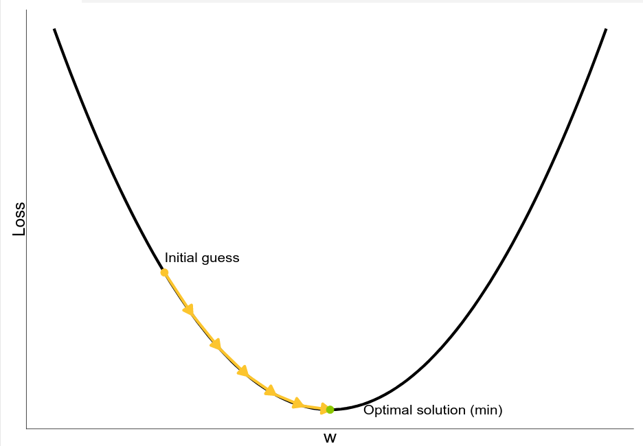
Source – Nicola Romanò – CC-BY-SA 4.0
If we have more than one parameter, we can use the gradient of the loss function to find the direction of the steepest descent. The gradient is a vector that points in the opposite direction of the steepest descent (technically, it is a vector of the partial derivatives of the loss with respect to each of the network variables). The gradient of the loss function is:
$$\nabla L = \left(\frac{\partial L}{\partial w_1}, \frac{\partial L}{\partial w_2}, \ldots, \frac{\partial L}{\partial w_n}\right)$$
The gradient descent algorithm can then be written as:
$$w_{i+1} = w_i – \alpha \nabla L$$
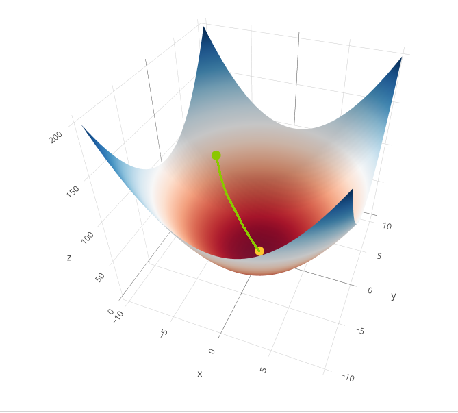
Source – Nicola Romanò – CC-BY-SA 4.0
We start with an initial guess $w_0$ and then update the guess using the following equation:
$$w_{i+1} = w_i – \alpha \frac{\partial L}{\partial w}$$
The learning rate is a key hyperparameter that controls how big the steps are in the gradient descent algorithm. If the learning rate is too small, the algorithm will take a long time to converge. If the learning rate is too large, the algorithm might not converge at all, so the choice of $\alpha$ is extremely important. Often we start with a large learning rate and then decrease it as the algorithm converges; this is called learning rate schedule.
Note that modern neural networks can have billions of parameters, so the situation is much more complicated there, but the basic principle is the same as in our 3D example!
Summary
In this and the last post, we have seen how ANN work, defined the building blocks of an ANN and how to train them using the gradient descent algorithm.
In the next post, we are going to build our first neural network using the Keras library in Python!