Build a simple neural network in Python!

In previous posts, we have looked at the theory of what is a neural network and how the training process works. Today we are going to put that into practice and build our own neural network using Python!

Requirements

For the example in this post, I will be using Python 3.10. We will build a neural network using keras from the tensorflow package.

TensorFlow is one of the most used solutions for building neural networks. In this post, we will be building a very simple one, but Tensorflow is extremely powerful and can be used to build complex neural networks. Using vanilla TensorFlow, however, can be a bit cumbersome. For this reason, we will be using Keras, which is a high-level API for TensorFlow. Keras is very easy to use and allows us to build neural networks in a few lines of code. While Keras used to be its own separate package, it is now part of TensorFlow.

There are a few other packages I will use; you can either install them separately or use this requirements.txt file to recreate a Python environment using:

pip install -r requirements.txt

The data

For this example, we are going to use the Wisconsin Breast Cancer dataset. This dataset is available on Kaggle, and contains data from 569 images of fine needle aspirates of breast masses. For each image, a series of ten features of the cell nuclei have been measured, along with whether the cancer is benign or malignant.

Let’s start with some exploratory data analysis (I assume you have placed it in the same folder as your Python script)…
We first read in the csv file, and print the names of the columns; you can see there are several features (e.g. area, smoothness, compactness etc) which have been calculated for each nucleus in the image; the file reports the mean, standard error and the “worst” or largest (mean of the three largest values) for each feature.

import pandas as pd
import matplotlib.pyplot as plt

wisconsin = pd.read_csv('data.csv')
print(wisconsin.columns)

Index(['id', 'diagnosis', 'radius_mean', 'texture_mean', 'perimeter_mean',
       'area_mean', 'smoothness_mean', 'compactness_mean', 'concavity_mean',
       'concave points_mean', 'symmetry_mean', 'fractal_dimension_mean',
       'radius_se', 'texture_se', 'perimeter_se', 'area_se', 'smoothness_se',
       'compactness_se', 'concavity_se', 'concave points_se', 'symmetry_se',
       'fractal_dimension_se', 'radius_worst', 'texture_worst',
       'perimeter_worst', 'area_worst', 'smoothness_worst',
       'compactness_worst', 'concavity_worst', 'concave points_worst',
       'symmetry_worst', 'fractal_dimension_worst'],
      dtype='object')

We can now check how many benign vs malignant cases there are; the dataset is relatively balanced, with ~63% of cases being benign.

print(wisconsin['diagnosis'].value_counts())

diagnosis
B    357
M    212
Name: count, dtype: int64

Finally, we can plot the mean features. We take advantage of the scatter_matrix functions from Pandas, which takes care of most of the “heavy lifting” for us.

from pandas.plotting import scatter_matrix

# Define a list of colours matching "purple" to malignant samples and "green" to benign
colors = ['green' if i=='B' else 'purple' for i in wisconsin['diagnosis']]

# Get only columns ending with 'mean'
mean_features = wisconsin[[c for c in wisconsin.columns if c.endswith('mean')]]

# Plot all columns ending with 'mean'
axes = scatter_matrix(mean_features, alpha=0.2, color=colors, figsize=(10, 10), diagonal='kde')
# Rotate axes labels 45 degrees
for ax in axes.flatten():
    ax.xaxis.label.set_rotation(45)
    ax.xaxis.label.set_ha('right')
    ax.yaxis.label.set_rotation(45)
    ax.yaxis.label.set_ha('right')

plt.show()

And here is the result!

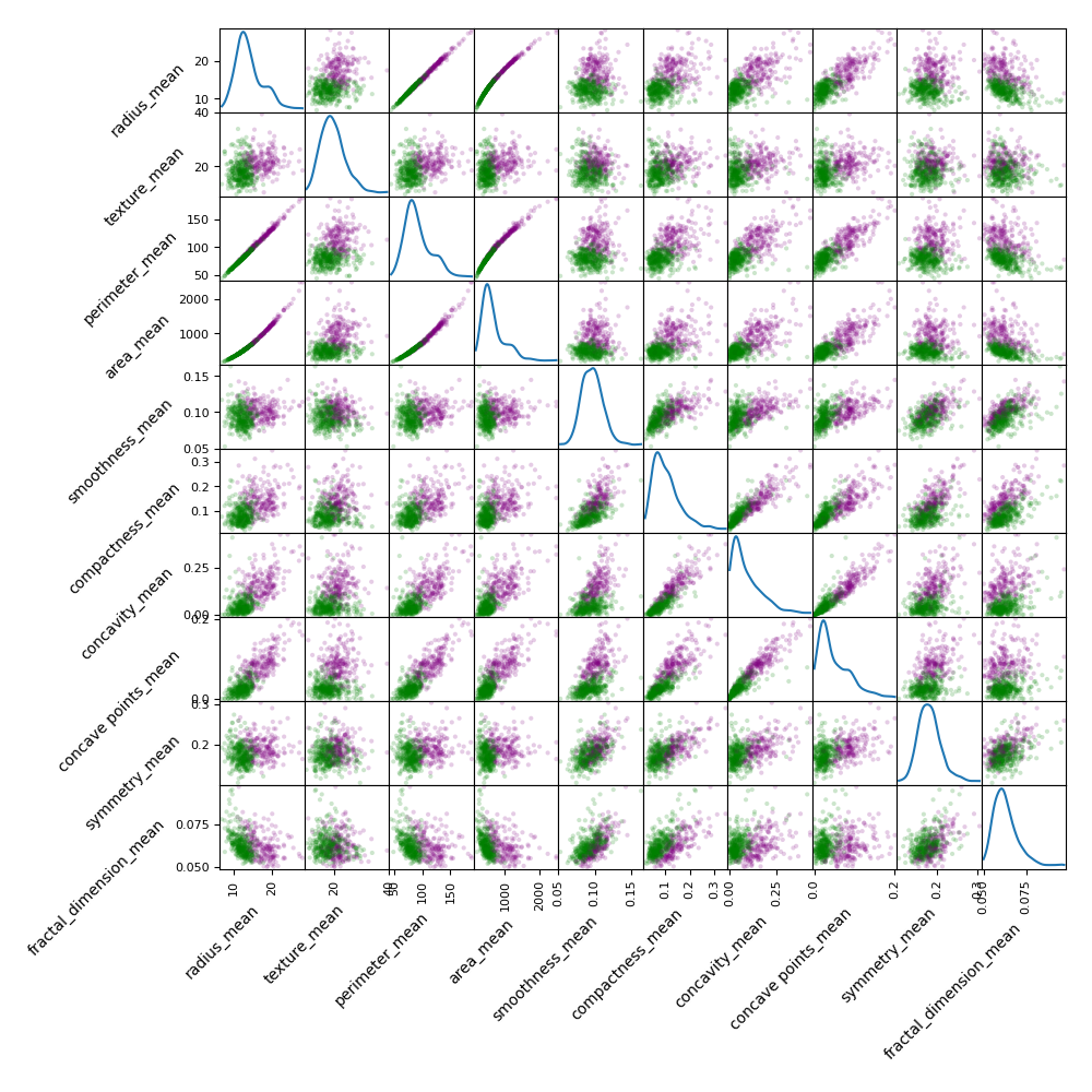
This tells us a lot!

The first thing to notice is that some features have very small values (e.g. smoothness, around 0.1), while others have very large values (e.g. area, with values around 1000). This is a problem, because neural networks are sensitive to the scale and the mean value of the input data (technically, they are not scale and shift invariant). If we don’t do anything, the neural network will learn to give more weight to the features with larger values, which is not what we want. We need to scale the data so that all features have a similar range. Other machine learning algorithms, such as decision trees, are scale and shift invariant, so they don’t need to be scaled.

Note that on the diagonal, we see the kernel density estimation (KDE) plots showing the distribution of each variable. Most variables have a normal (-ish) distribution, often with a bit of tail on the right. In some cases the distribution is clearly not normal, but this is not a problem. Remember that ANN are universal function approximators, so they can learn to fit any distribution, and correction for non-normality is not necessary.

Looking at the scatterplots, we see that this particular classification problem is easily and possibly linearly solvable. Indeed in most cases you can separate the green and the purple points with a single line, so a neural network should be able to do the same.

Finally, some of the features, such as area and perimeter, are highly correlated. This is not a problem, because neural networks are able to learn to ignore (or even to exploit!) redundant features.

Data preparation

We start by loading the data and splitting it into a training set (70%), a validation set (20%) and a test set (10%). We use the training set to train the neural network, and the validation set to evaluate its performance during training. Finally, we use the test set to evaluate the performance of the neural network after training. Importantly, we do not use the test set at all during training; this is only used at the very end to evaluate the performance of the neural network.

It is important not to use the same data during training and testing. If we did, we would be using the test set to improve the neural network during training, and then we would be using the same test set to evaluate the performance of the neural network. This would give us an overly optimistic estimate of the performance of the neural network. This is called information leakage, and it is a common mistake in machine learning.

We will use StandardScaler to scale the data, which scales the data to have zero mean and unit variance. Again, we only fit the scaler on the training set, and then use the same scaler to transform all sets, to avoid information leakage. We also convert the outcomes to numbers, setting “M” (malignant) to 1 and “B” (benign) to 0. The order of this factor is arbitrary, and we could have assigned 0 to “M” if we wanted without affecting the final result.

from sklearn.model_selection import train_test_split
from sklearn.preprocessing import StandardScaler

all_features = wisconsin.drop(['id', 'diagnosis'], axis=1)
# The train_test_split function only splits into two groups, so we need to call it twice to get three groups!
# Split 70/30
x_train, x_val, y_train, y_val = train_test_split(all_features, wisconsin['diagnosis'], test_size=0.3, random_state=42)
# Split the 30 into 66/33, giving us a 70/20/10 split
x_val, x_test, y_val, y_test = train_test_split(x_val, y_val, test_size=0.33, random_state=42)

# Scale the data
scaler = StandardScaler()
x_train = scaler.fit_transform(x_train)
x_val = scaler.transform(x_val)
x_test = scaler.transform(x_test)

# Convert labels to numbers
y_train = y_train.map({'M': 1, 'B': 0})
y_val = y_val.map({'M': 1, 'B': 0})
y_test = y_test.map({'M': 1, 'B': 0})

As a sanity check, we can print the shape of the training and test set

print(f"Training set: {x_train.shape}")
print(f"Validation set: {x_val.shape}")
print(f"Test set: {x_test.shape}")

Training set: (398, 30)
Validation set: (114, 30)
Test set: (57, 30)

We can also check that the data has been scaled correctly by printing the mean and standard deviation of each feature. The mean should be 0 (in reality, it is a very small value), and the standard deviation should be 1.

train_mean = x_train.mean(axis=0)
train_std = x_train.std(axis=0)
print(f"Mean: {train_mean}")
print(f"Standard Deviation: {train_std}")

Mean: [ 2.67792488e-16 -5.53437809e-16 -6.18154327e-16  2.07539178e-16
  8.92641628e-18 -9.59589750e-17 -2.09770783e-16 -1.35012046e-16
  7.25271323e-16  2.80066311e-16  1.22738224e-16  6.24849139e-17
  3.25814194e-16 -1.45054265e-16  2.36550031e-16  3.12424570e-17
 -5.57901017e-17 -2.58866072e-16  9.14957669e-17  3.79372692e-17
  5.95838287e-16 -1.98612762e-16 -3.01266549e-16 -1.65138701e-16
  9.10494460e-16 -1.74065117e-16  1.29433036e-16  8.70325587e-17
 -2.73371499e-16  1.42822660e-16]
Standard Deviation: [1. 1. 1. 1. 1. 1. 1. 1. 1. 1. 1. 1. 1. 1. 1. 1. 1. 1. 1. 1. 1. 1. 1. 1.
 1. 1. 1. 1. 1. 1.]

Let’s build the neural network!

We will use the Sequential model, which is the simplest model in Keras, to create a network with an input layer, a hidden layer, and an output layer. The input layer accepts the 30 features, the hidden layer has 10 nodes, and the output layer has a single node, which is the predicted probability of the cancer being malignant (because we assigned 1 to malignant).

Note that a Dense layer in Keras implies a fully connected layer, that is, each node in the layer is connected to each node in the previous layer. Keep this in mind if using a lot of layers and/or nodes, because that makes the number of parameters the net needs to estimate grow very quickly!

We use the ReLU activation function for the hidden layer, and the sigmoid activation function for the output layer, since this is a binary classification problem.

from tensorflow.keras.models import Sequential
from tensorflow.keras.layers import Dense, InputLayer
from tensorflow.keras.utils import plot_model

# Define the model
model = Sequential()
model.add(InputLayer(input_shape=(x_train.shape[1],)))
model.add(Dense(20, activation='relu'))
model.add(Dense(1, activation='sigmoid'))

# Print a summary of the model
print(model.summary())
# Plot the model
plot_model(model, show_shapes=True)

Model: "sequential"
_________________________________________________________________
 Layer (type)                Output Shape              Param #   
=================================================================
 dense (Dense)            (None, 20)                620       
                                                                 
 dense_1 (Dense)            (None, 1)                 21        
                                                                 
=================================================================
Total params: 641
Trainable params: 641
Non-trainable params: 0
_________________________________________________________________
None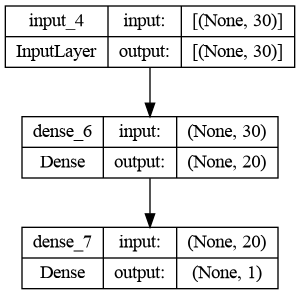

This is a very simple network; the first layer has 620 parameters (30 features going onto 20 nodes, using 30 * 20 = 600 weights + 20 biases = 620 parameters in total) and the output layer only uses 20 weights from the 20 neurons of the hidden layer + 1 bias. Modern complex neural networks can have even trillion parameters!

We now specify that we will use the binary cross-entropy loss function; we will use Adam, a commonly used optimizer (the algorithm that will be used to minimize the loss function). Finally, we define which metrics we want to track. We use accuracy, which is the fraction of correctly classified samples (true positives and true negatives).

model.compile(optimizer='adam', loss='binary_crossentropy', metrics=['accuracy'])

We now call model.fit to train the network. At each epoch, the loss and the metrics will be computed on both the training and the validation data (but the network is only trained on the training data). The result of training for, in this case, 50 epochs, will be stored in the history variable, which will contain values for the loss and for any metrics we specified when compiling the model.

history = model.fit(x_train, y_train, validation_data=(x_test, y_test), epochs=50)

Epoch 1/50
15/15 [==============================] - 0s 8ms/step - loss: 0.5002 - accuracy: 0.7495 - val_loss: 0.4480 - val_accuracy: 0.7895
Epoch 2/50
15/15 [==============================] - 0s 3ms/step - loss: 0.4353 - accuracy: 0.8132 - val_loss: 0.3866 - val_accuracy: 0.8684
Epoch 3/50
15/15 [==============================] - 0s 2ms/step - loss: 0.3860 - accuracy: 0.8681 - val_loss: 0.3393 - val_accuracy: 0.8947

...
[output cut]
...

Epoch 49/50
15/15 [==============================] - 0s 3ms/step - loss: 0.0648 - accuracy: 0.9868 - val_loss: 0.0599 - val_accuracy: 0.9825
Epoch 50/50
15/15 [==============================] - 0s 3ms/step - loss: 0.0640 - accuracy: 0.9868 - val_loss: 0.0595 - val_accuracy: 0.9825

We can now plot the loss and accuracy during training

fig, ax = plt.subplots(1, 2, figsize=(10, 5))
ax[0].plot(history.history['loss'], label='loss')
ax[0].plot(history.history['val_loss'], label='validation loss')
ax[0].legend()
ax[0].set_title('Loss')
ax[1].plot(history.history['accuracy'], label='accuracy')
ax[1].plot(history.history['val_accuracy'], label='val_accuracy')
ax[1].legend()
ax[1].set_title('Accuracy')

plt.show()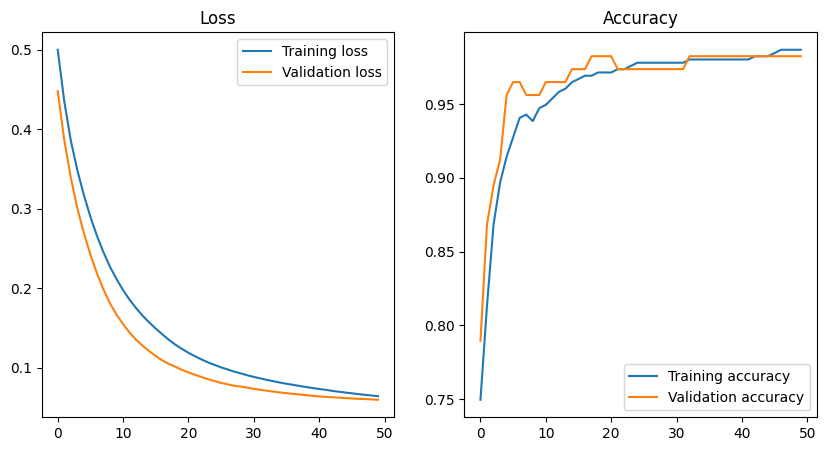

This is pretty much a textbook example of loss and accuracy curves. The loss decreases, and the accuracy increases towards 1 with the number of epochs. Importantly, the loss and accuracy curves for the training and validation data are very similar; remember that the validation data is not used to train the network, so this means that the network is able to generalize well to unseen data and it is not just memorizing the training data (overfitting).

We can now evaluate the performance of the model on the test set

print(model.evaluate(x_test, y_test))

2/2 [==============================] - 0s 3ms/step - loss: 0.0308 - accuracy: 0.9825
[0.03076927736401558, 0.9824561476707458]

Predicting new data points!

OK, so now we have a neural network… what do we do with it? Well, we could gather new data using the same method and calculating the same features, and use our model to predict whether it is from a benign or a malignant tumour!

We will use the predict function, which will return the probability of the tumour being malignant. We can then use a threshold of 0.5 to classify the tumour as benign or malignant. Note that the choice of threshold is important, and this should be tuned depending on the balance of false positives and false negatives that you want to achieve. For example, if you want to minimize the number of false negatives (i.e. you want to be sure that you don’t miss any malignant tumour), you should use a threshold that is lower than 0.5. This will increase the number of false positives, but it will reduce the number of false negatives.

predictions = model.predict(x_test)
# Print the first 5 predictions
print(f"Probabilities:\n{predictions[:5]}")
# Convert predictions to either 0 or 1
predictions = np.where(predictions > 0.5, 1, 0)
print(f"Thresholded predictions:\n{predictions[:5]}")

2/2 [==============================] - 0s 2ms/step
Probabilities:
[[2.2237592e-07]
 [2.3205655e-03]
 [1.6656233e-05]
 [9.9999988e-01]
 [6.1853875e-06]]
Thresholded predictions:
[[0]
 [0]
 [0]
 [1]
 [0]]

A useful way of visualizing how the model performs is to use a confusion matrix, which shows a comparison between the real data and the predictions of the model.

Note that we can only do this because we are using the test set, for which we know the true labels. If we were predicting completely new data, we would not be able to create a confusion matrix.

import seaborn as sns
from sklearn.metrics import confusion_matrix
print(np.unique(y_test, return_counts=True))
cm = confusion_matrix(y_test, predictions)
sns.heatmap(cm, annot=True, cmap='Blues')
plt.xlabel('Predicted')
plt.ylabel('Truth')
plt.show()

OK, this seems to work almost perfectly, with only one misclassified sample (a benign tumour classified as malignant). However, remember what we said at the very beginning; this is a simple, almost linearly separable problem. In reality, things are often more complicated… but that is a topic for another post!