
In this series of posts I will introduce one of the simplest, yet very powerful statistical models, linear regression. We’ll start with some theory, then move on to a few practical examples in R.
The basic theory
Not interested in the maths? Skip to the examples!
Linear regression is part of the larger family of statistical models called linear models. It models an outcome continuous variable as a linear combination of one or more so-called explanatory variables, or predictors. If we have only one predictor, we talk about simple linear regression; in this case, our model simply reduces to fitting a line to our data. If we had two predictors, we would be modelling a plane and for multiple predictors a hyper-plane (which is something slightly difficult to imagine).
Mathematically, if we model $Y$ as a function of n predictors $X_1$ to $X_n$, we will have
$$Y_i = \beta_0 + \beta_1 X_{1i} + \beta_2 X_{2i} + … + \beta_n X_{ni} + \epsilon_i$$
The coefficients $\beta$ multiply each of the predictors, and so act as weights and tell us how much each X is important to determine Y. A coefficient of 0, indicates no effect of the predictor on the outcome. A positive coefficient indicates a positive impact of the predictor (i.e. when the predictor increases, the outcome increases). In contrast, a negative coefficient shows a negative effect of the predictor on the outcome.

$\beta_0$ is called the intercept and simply represents the value of the outcome when all the predictors are 0. Finally, we also add an error or residual term $\epsilon$, which is the difference between what our model predicts and what our real data actually is. Linear regression assumes that the errors $\epsilon$ come from a normal distribution $N(0, \sigma)$ (more on that later).
Often you will find the equation above written in matrix form, which is useful especially for complex models with a large number of predictors. So, for a model with $k$ predictors $X_1$ to $X_k$ and $n$ observation we would have
$$\mathbf{Y}=\mathbf{\beta} \mathbf{X}+\mathbf{\epsilon}\tag{2}\label{eq2}$$
Which is the short form for this ugly thing down here…
$$\begin{bmatrix}
Y_1\\ Y_2\\ \vdots \\ Y_n\
\end{bmatrix} =\begin{bmatrix} 1 & X_{1_1} &… & X_{k_1} \\ 1 & X_{1_2} &… & X_{k_2} \\ \vdots & \vdots & \ddots &\vdots\\ 1 & X_{1_n} &… & X_{k_n} \end{bmatrix} \begin{bmatrix}
\beta_1\\ \beta_2\\ \vdots \\ \beta_k\
\end{bmatrix} + \begin{bmatrix}
\epsilon_1\\ \epsilon_2\\ \vdots \\ \epsilon_n\
\end{bmatrix}$$
So, our goal is to estimate the $\beta$ coefficients, in order to best fit our data. What the best fit is can depend on the situation, but mostly we consider best the line that minimises the sum of squares of the residuals $\epsilon$, usually done using the ordinary least squares (OLS) method. So we want to minimize:
$$\sum_{i}{(y_{predicted_i} – y_i)^2}$$
By squaring the residuals we ensure that all terms of the sum we are minimising are positive.
But, enough talk… let’s dive into an example!
A simple example
Consider this very simple dataset, containing core body temperature measurements for 34 male subjects of different age. We want to ask the question of whether age affects temperature, and we would like to be able to predict the core body temperature of a new subject just by knowing their age.
Basic data exploration
We can start by reading the dataset and plotting the data
library(ggplot2)

# Read data from the csv file
temp <- read.csv("temperature.csv")
# Scatterplot of Age vs Temperature
ggplot(data = temp, aes(x = Age, y = Temperature)) +
  geom_point()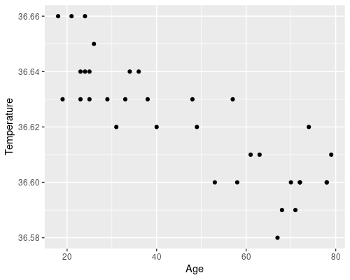
There is an evident downward trend of temperature with age. There are also some biological reasons to believe that age could affect temperature, which makes our idea of somehow using a statistical model to link the two at least reasonable.
Generating the model
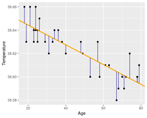
This is a case of simple linear regression, modelling the Temperature outcome as a linear function of one explanatory variable, Age. So
$$\mathbf{Temperature} = \beta_0 + \beta_1 \mathbf{Age} + \mathbf{\epsilon}$$
Essentially we want to find a line, such as the orange one in the following figure. The residuals (i.e. the differences between the original data point and the fitted values) are drawn in blue.
In R, defining this linear model is super easy, by using the lm function!
model <- lm(Temperature ~ Age, data = temp)That’s it! But before we go and have a look at the model’s result we need to check that the assumptions of linear regression are satisfied.
Assumptions of linear regression
There are several assumptions that need to be checked:
- Random sampling
- Independence of measurements
- Homogeneity of variance (also called homoscedasticity)
- Normality of residuals
Random sampling relates to data collection, so we cannot deal with that here, but we will assume that is satisfied.
We also know that measurements are independent, as each of them comes from a different individual. Obviously, there could be other sources of non-independence, but we will ignore them here. I will talk about dealing with non-independent measurement in another post!
Testing homogeneity of variances
The other two assumptions can be tested by looking at the residuals. The easiest way is to use the “diagnostic plots” obtained by plotting the model. Calling plot on a lm model will produce four plots; passing the which argument allows us to only plot the ones we are interested in (in this case 1 and 2).
plot(model, which = 1)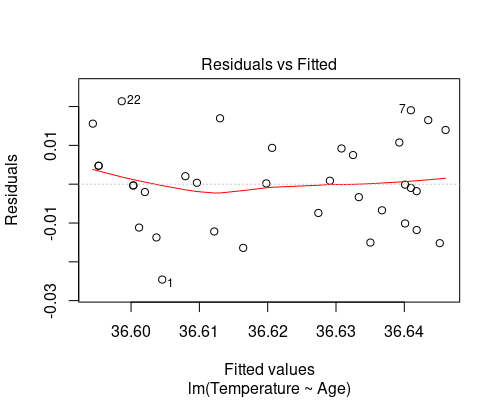
The first plot (fitted vs residuals) shows how residuals vary over the range of fitted values. Residuals greater than 0 correspond to data points above the fitted line, while residuals below 0 correspond to data points below the fitted line, as exemplified in the graphs below.
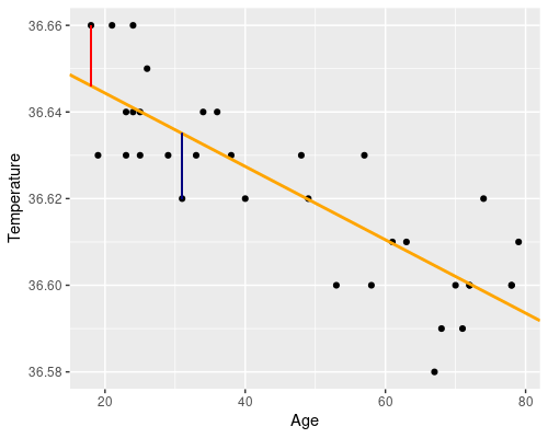
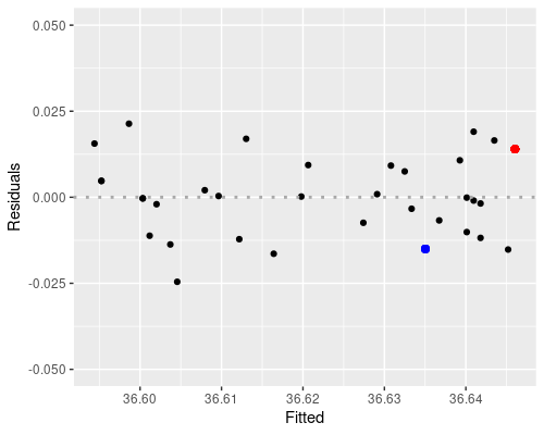
the blue point is above, so its residual is positive.
The residuals vs fitted plot shows no particular trend, and it tells us that essentially our data points are equally spread throughout the range of fitted values. This indicates homoscedasticity, that is, uniformity of the variance throughout the range of fitted values.
Below you can see two examples of fitted vs residuals plots that indicate non-uniform variance. In both of these cases, we should not rely on our linear model, as its assumptions would not be met. We will see how to deal with these cases in another post.
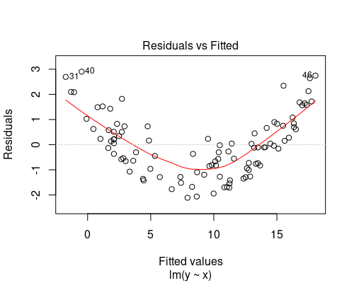
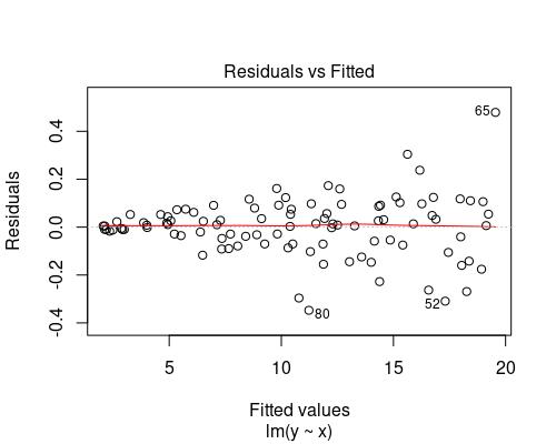
The plot on the top indicates some non-linearity in the relationship between the variables, while the one at the bottom shows residuals getting larger as fitted values increase.
Testing normality of residuals
The second diagnostic plot is a QQ plot of the residuals.
plot(model, which = 2)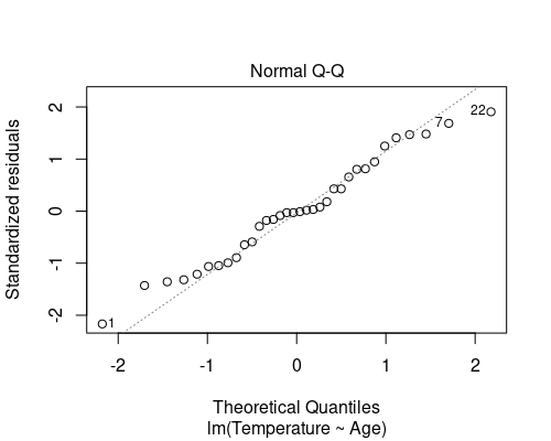
This QQ plot shows the quantiles of our residuals against those of a normal distribution. If the residuals are normally distributed, points will follow the dotted line. In general, especially for the larger residuals, some deviation from normality is often seen (as in this case), and it is not necessary to deal with it; linear regression is indeed robust to small deviations from normality.
The QQ plot suggests that the last assumption is also met.
Note: personally, I like to rely on visual inspection of these plots to evaluate if assumptions are met. You could, however, check assumptions in other ways. For instance, you could run a formal normality test, such as the Shapiro-Wilk test, or plot the histogram of the residuals. Similarly, you can run a variance test to check for homoscedasticity. You can easily retrieve the residuals of a model using
model.resid <- resid(model)Evaluating the results
OK, finally after all of this we can look at the results of our model!
summary(model)Call:
lm(formula = Temperature ~ Age, data = temp)
Residuals:
Min 1Q Median 3Q Max
-0.0245619 -0.0094385 -0.0002212 0.0087750 0.0213632
Coefficients:
Estimate Std. Error t value Pr(>|t|)
(Intercept) 3.666e+01 4.922e-03 7448.492 < 2e-16 ***
Age -8.465e-04 9.632e-05 -8.787 4.85e-10 ***
---
Signif. codes: 0 ‘***’ 0.001 ‘**’ 0.01 ‘*’ 0.05 ‘.’ 0.1 ‘ ’ 1
Residual standard error: 0.01168 on 32 degrees of freedom
Multiple R-squared: 0.707, Adjusted R-squared: 0.6979
F-statistic: 77.22 on 1 and 32 DF, p-value: 4.85e-10That is a lot of information! Let’s walk through that, bit by bit.
At the top, we get our model formula and a summary of the residuals. This can be used as a further back of the envelope residual normality check, by checking that the median is ~0 and the distribution is symmetrical.
The estimated coefficients
We then get the estimations of the $\beta$ coefficients. Specifically, we get:
$\beta_0$ (the intercept) = 36.66. This is the core temperature corresponding to an age of 0. Although probably not biologically meaningful in this case, interpreting the intercept is very useful in other models.
$\beta_1$ = -0.00084. This is the slope for Age. This means that core body temperature decreases of 0.00084 degrees for every year of age.
These values are calculated from our sample, so they are estimates, and they are associated with an error, which is reported next to each coefficient.
The (dreaded) p-values
We then have a t-statistics and a corresponding p-value.
To understand this, we need to think about what linear regression is actually testing. The null hypothesis of linear regression is that $\beta = 0$, that is, the predictor (Age) does not influence the outcome (Temperature).
The t-statistics is calculated dividing the estimated coefficients by their standard error. The p-value gives us the probability of getting t statistics as high or larger (in absolute value) than the one obtained if the null hypothesis $H_0$ is true.
In other words, since the p-value for age is extremely small we can refute the null hypothesis that Age does not have an effect on core body temperature. The p-value of $10^{-10}$ means that there is a very low probability of $10^{-10}$ of obtaining t statistics as big as -8.787 if Age had no effect.
We can easily plot the results of our model
# Retrieve the model coefficients
cf <- coef(model)

ggplot(temp, aes(Age, Temperature)) +
  geom_point() +
  geom_abline(intercept = cf[1], slope = cf[2],
              col = "red", lwd = 1.5)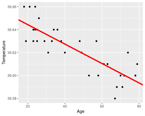
How good is your model?
Finally, let’s look at the final part of the summary
Residual standard error: 0.01168 on 32 degrees of freedom
Multiple R-squared:  0.707,	Adjusted R-squared:  0.6979
F-statistic: 77.22 on 1 and 32 DF,  p-value: 4.85e-10
This gives us an estimation of the standard deviation of the normal distribution the residuals are drawn from (residual standard error), and the degrees of freedom of our model, equal to the number of observation minus the number of parameters.
Multiple $R^2$, is a measure of how well the model fits the data; it goes from 0 to 1 (perfect fit). In our case, $R^2 = 0.707$ means that 70.7% of the variability of the data is explained by our predictors. The rest of the variability is left in the residuals. To better understand this, we can try to calculate $R^2$ by ourselves. Consider the mean temperature $\bar{T}$; we can calculate the sum of squares of the differences between the fitted values $\hat{T}$ and the mean $\sum{(\hat{T}-\bar{T})^2}$. This is a measure of the variability explained by our model. We compare that to the total variability $\sum{(T-\bar{T})^2}$, calculated on the measured data. In R:
sum((model$fitted.values - mean(temp$Temperature))^2) /
   sum((temp$Temperature - mean(temp$Temperature))^2)
[1] 0.7070096If we were to add a new predictor to the model, even if that predictor were completely unrelated to the outcome, we would increase $R^2$. Obviously, this is not desirable, but we can correct for the model complexity, and that is what the adjusted $R^2$ is.
At the very bottom, we get an F statistic and associated p-value. These are a measure of fit for the whole model, testing the null hypothesis that all coefficients are 0. In the case of simple linear regression, this is trivial, since we only have one predictor.
And that’s it for this post! Part 2 will deal with multiple predictors, including discrete ones, and how to deal with interactions!