This is the first of a series of posts where I will introduce you to neural networks. Even if you do not know how they work, you have probably heard of neural networks in the news as something used for artificial intelligence. Many areas, such as image recognition, natural language processing, fraud detection and many more (biology included!), have taken incredibly huge steps forward in the last few decades thanks to these techniques, and the number of applications for neural networks is increasing exponentially.
For example, the image at the top of this page has been generated by a neural network!
In this series, I will guide you through understanding neural networks, starting from very simple ones to some of the more complex and powerful types used today. In later posts, we will use Python to create neural networks.
So, let’s dive into this fascinating topic!
What is a neural network, anyway?
An artificial neural network (ANN), or neural networks for short, is a construct used to perform computations in various machine learning problems. Just like a biological neural network, it is made up of a series of “artificial neurons” connected to each other. Each neuron of an ANN can receive signals and, after processing them, generate an output that it feeds to other neurons.
While it is compelling (and makes good PR stunts!) to make comparisons between biological and artificial neural networks, they have many differences that are outside of the scope of this post, I am afraid!
A brief history of neural networks
The McCulloch-Pitts neuron
It was 1943 when Warren S. McCulloch and Walter Pitts published their seminal article “A logical calculus of the ideas immanent in nervous activity“. In this paper, they propose a basic model of a neuron, which is known today as the McCulloch-Pitts (MP) neuron. Let’s see how it works!
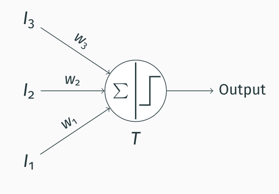
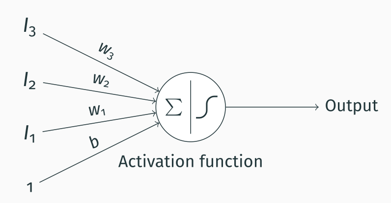
The MP neuron is extremely simple. The idea is that it receives inputs (in the figure above, you can see 3 inputs $I_n$) and weights them with different weights ($w_n$). These inputs are then summed, and the result is thresholded. This is somehow resemblant to how a biological neuron receives multiple inputs of different strengths (=different weights) from other neurons, and it integrates these inputs to generate a response (=output).
So basically we have $$\sum_{i=1}^{3}I_i * w_i > T$$
or, without any fancy math notation $$I_1 * w_1 + I_2 * w_2 + I_3 * w_3 > T$$
MP neurons only accept 0 or 1 as inputs and +1 or -1 as weights (representing a stimulatory or an inhibitory input, respectively), so their applications are fairly limited; however, while they hardly have any practical use today, they formed the basis for modern neural networks.
The perceptron
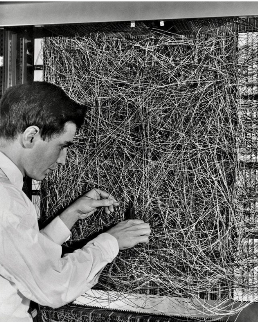
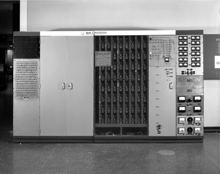
We need to wait until 1958 to really see some ANN which found practical use with the advent of the perceptron. The perceptron was developed in 1958 by Frank Rosenblatt and was meant to be used by the US Navy for image recognition. The perceptron is still fairly limited in what it can do, but it was a step up from what we saw for MP neurons.
Similarly to MP neurons, the perceptron is a binary classifier, which takes a series of inputs and linearly combines them to generate an output. Below is a depiction of how a perceptron works.
You can see that the perceptron is fairly similar to the MP neurons, with some important differences. We add an extra input with a fixed value of 1 and weight $b$; this is called the bias and allows us to offset the sum of the inputs. You can see that the sum now becomes $$\sum_{i=1}^{3}I_i * w_i + b$$
Activation functions
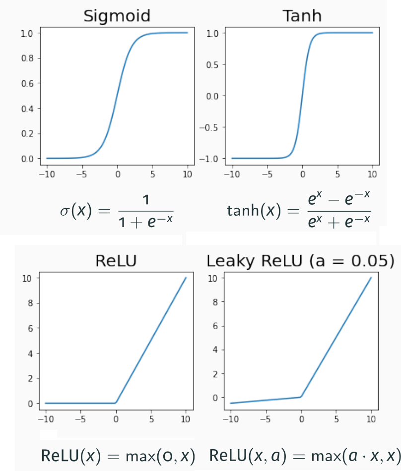
The other significant difference in the perceptron is that instead of a simple threshold, we use an activation function. In the case of the perceptron, this is a sigmoid (with equation $y=\frac{1}{1+e^-x}$). The activation function allows us to introduce non-linearities so that we can capture more complex relationships between the inputs and the output.
Other non-linear functions can be used as activation functions. One of the most commonly used nowadays is the Rectified Linear Unit (ReLU); this is computationally fast to calculate and has mathematical properties that make it an attractive choice for neural networks.
The perceptron – a practical example
I will now give a practical example of how a perceptron could be used. Let’s say we have a perceptron that allows us to classify data into two classes (e.g. correct/incorrect or dog/cat or illness/no illness, etc.). We do so by passing three relevant variables (or features) to the perceptron, as shown in the figure below. For instance, if we wanted to classify whether a patient has some illness, we might pass the amount of three substances in the patient’s blood, their age, whether they smoke and so on.
For this example, we assume that somehow we have already calculated the optimal weights for this task; we will discuss how to do that in the next part.
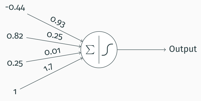
Now what we have to do is sum the weighted inputs getting $$\sum_{i}I_i * w_i + b = 0.25 * 0.01 + 0.82 * 0.25 − 0.44 * 0.93 + 1.7 = 1.498$$
We now pass the result through the activation function $$\frac{1}{1 + e^{−1.498}} = 0.9$$
As I said, the perceptron is used for binary classification, so we need to go from $0.9$ to our binary output. We do this employing a simple thresholding process. For example, we can say that anything $>=0.5$ corresponds to illness, and anything $<0.5$ corresponds to no illness. So, in this case, the sample comes from someone with the disease.
Side note: if you are into statistics, you have probably recognised this as your friend, the logistic regression! Well, it is not quite the same thing, although, in practice, both models will eventually come to the same conclusion.
Extending the perceptron – the multi-layer perceptron
The perceptron is great for solving simple tasks but is still somehow limited in what it can do. We can extend the idea of the perceptron by sequentially connecting multiple neurons by generating layers of perceptrons. This is called a multi-layer perceptron (MLP) and allows for solving much more complex problems. MLP are universal function approximators that can be proven to approximate any mathematical function, so any mathematical relationship between inputs and outputs. So much so that most modern neural networks, even the very complex and powerful ones, contain MLP as part of their processing pipeline.
So, what does an MLP look like?
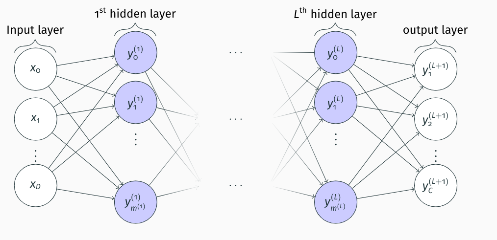
As you can see in the figure, we still have our inputs and outputs, but we process them through a network of connected perceptrons arranged in layers. There can be an arbitrary number of hidden layers between the inputs and the outputs, but the basic calculations are always the same.
- We start from the first hidden layer.
- We calculate the output of each neuron as the weighted sum of the inputs plus the bias.
- We pass the result through the activation function
- The output of this neuron is used as input for neurons in the next hidden layer until we reach the output layer
You can see that in this example, not only do we have multiple inputs but also multiple outputs! Indeed, MLP can be used to generate numerous responses at the same time.
Multi-class classification problems
Finally, this post would not be complete without a note on classification problems. The networks described so far work well in the case of regression problems (i.e. predicting a continuous value from a set of features, say the price of a house given its location, number of rooms, etc.) or for binary classification problems (e.g. when predicting whether a patient has a disease or not).
Often, however, we want to predict multiple classes (e.g. given an image of a chest X-ray, we want to predict whether it’s from a patient with no disease, with pneumonia or with tuberculosis). This is called a multi-class classification problem. We saw that the sigmoid function can be used for binary classification since we can obtain 0/1 outputs by thresholding it. However, it is not suitable for multiclass classification.
In these cases, we can use a generalization of the sigmoid called softmax. The softmax function is defined as follows:
$$\sigma(z)_j = \frac{e^{z_j}}{\sum_{k=1}^Ke^{z_k}}$$
The softmax function is a vector of probabilities summing to 1, so that the $j$-th element of the softmax function is the probability that the input belongs to the $j$-th class. In the next posts, we will come back to the softmax and see how it is used in practice.
Summary
Hopefully, you now have an idea of what are the building blocks of a neural network and of its basic functioning.
But, I hear you ask, this is all nice and good, but how do I choose my neural network’s parameters (weight and biases)? Well, that is the next post‘s topic, so stay tuned!