Easy methods for segmentation of biological images.

In the previous two posts we saw how to use Scikit Image to perform some basic image processing. This post will introduce you to image segmentation, one of the most important steps in image analysis. I am going to cover some of the “traditional” methods that work well in many situations. These methods require adaptation (or don’t work at all!) for more complex cases… but that is maybe a story for another post!

Introduction

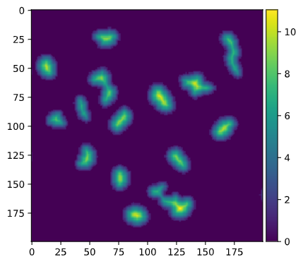
Segmentation is the process of dividing a digital image into subsets of pixels with certain features. This is used, for instance, to determine where specific objects are in an image. Depending on the use case, there are different types of segmentation, as shown in the image below.

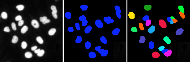
In the image above, we see some cell nuclei. We can perform a simple segmentation by assigning to each pixel a value of 0 if they are in the background or 1 if they are in a nucleus. This is called semantic segmentation, and is a useful technique, for instance, to determine cell density. Often, however, we want to know where each nucleus is, for example, to count the number of cells, or to determine their size, position, intensity and so on. This is the case of the image on the right, where we separated each instance of the nuclei, and marked it with a different colour; this is called instance segmentation.

Semantic segmentation

Semantic segmentation is the easiest type of segmentation to perform. There are many methods that can be used, depending on the type of image you are using. In the case of microscopy fluorescence images, the easiest and most widely used technique is thresholding. Essentially we decide on an intensity level which we use to classify our pixels. So, if we are dealing with an 8-bit image and our threshold is 80, every pixel with intensity greater than 80 is classified as foreground, and everything else is background.

Let’s try it!

from skimage.io import imread, imshow

img = imread("nuclei.tif")
img_thresh = img>80

If you were to print img_thresh you would see something like

[[False False False ... False False False]
 [False False False ... False False False]
 [False False False ... False False False]
 ...
 [False False False ... False False False]
 [False False False ... False False False]
 [False False False ... False False False]]

Basically, we get a value of True or False depending on whether the pixel is above or below our threshold. We can use imshow to visualize this mask.

imshow(img_thresh)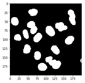

Choosing the threshold

In the example above I manually chose a threshold of 80, by simply guessing it from the image. This is obviously not the optimal solution, especially if we are processing a large number of images that may be different in overall intensity. A commonly used algorithm to select a threshold in these situations is Otsu’s thresholding method. This method returns an intensity value that maximises the variance between the two classes of pixels or, conversely, that minimizes the intra-class variance (see the Wikipedia page for a mathematical treatment). Otsu’s tresholding is implemented in skimage.filters.

from skimage.filters import threshold_otsu

thr = threshold_otsu(img)
print(thr)

113

Using Otsu’s method we found that the optimal value of threshold for this image is 113, slightly higher than what we previously had guessed. Let’s visualise it

img_thresh_otsu = img > thr
imshow(img_thresh_otsu)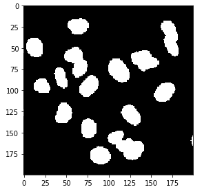

Although the result looks very similar to what we obtained before we can see that the cells are captured better. We can easily visualize the difference between the two results (note that since we are dealing with booleans I use the ^ operator rather than -.

imshow(img_thresh ^ img_thresh_otsu)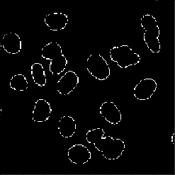

Other methods

Sometimes, images may not be uniform, and a single threshold may not be enough for segmenting. Scikit Image has various other options for thresholding, in the filters submodule, such as threshold_local. This creates a pixel-wise threshold based on each pixel’s neighbourhood (also called adaptive threshold). Another interesting option, when there are more classes of objects (e.g. bright cells, dim cells and background) is to use threshold_multiotsu , which is a generalisation of Otsu’s method for multiple classes. The filters manual page explains all these methods in detail.

Instance segmentation

Instance segmentation is a much more complex matter. I am going to cover only one simple solution, using a technique called watershed.

The main idea is to first create a binary mask of our image, as seen above, then identify the center of each cell and use that as a “seed” to divide the mask into instances.

Let’s see how to do it with Scikit Image

from scipy.ndimage import distance_transform_edt

distance = distance_transform_edt(img_thresh_otsu)

We use the distance_transform_edt from Scipy to find the Euclidean distance of each point of the mask from the background. This looks like this

We can now proceed to the watershed

from skimage.feature import peak_local_max
from skimage.measure import label
from skimage.segmentation import watershed
from skimage.filters import median
from matplotlib.colors import ListedColormap

# Find the local maxima of the distance map.
# Impose a minimum distance of 10 and use a "footprint"
# of 3x3 to search for local maxima
local_maxima = peak_local_max(distance, min_distance=10,
               footprint=np.ones((3, 3)), indices=False)

# Label connected regions
markers = label(local_maxima)
segmented = watershed(-distance, markers, mask=img_thresh_otsu)

# Use ListedColormap to create a random colormap to
# help visualize the results
cmap = ListedColormap(np.random.rand(256,3))
imshow(segmented, cmap=cmap)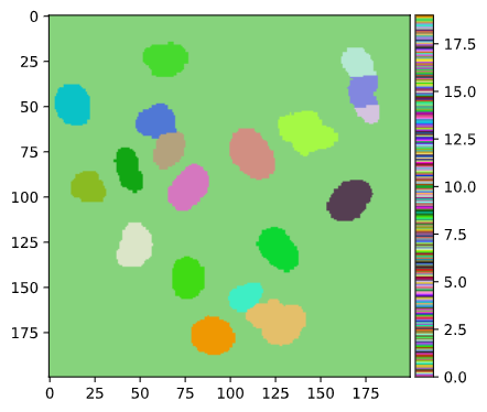

Some final thoughts

We’ve just scratched the surface here and there are many situations where these techniques will fail. As you can see, even what we could consider as a simple image, such as the one above poses some issues.

Finally, a note on 3D images; while these techniques also work on 3D images, they need some substantial tweaking in most situations and are not necessarily guaranteed to work there. There is a lot of interesting research on the topic and new approaches, for instance using convolutional neural networks, are constantly improving. Hope you enjoyed this post and keep in touch for more!