In the first part of this series, we looked at how to open images and perform some basic manipulations using Scikit Image. This second part will introduce you to digital image filters!
Digital filters for image analysis
Often we need to perform some operation on our images. For example, we may want to reduce noise, find object edges in the image. Digital filters can help with that!
In image analysis, a digital filter is a mathematical operation that is applied to the image to perform specific operation on it. The output image results from the application of said operation in a pixel-wise manner on the input image.
Usually we apply the operation to a region around each pixel of interest, most often square or rectangular; we then slide this region throughout the image to apply the operation to each pixel. This sliding window is called the filter kernel.
Simple filters: min, max, mean, median
These are probably the simplest examples of filters. They consist of a $n \times m $ kernel that “moves” through the image and applies a specific operation (e.g. the minimum) to the neighbourhood of each pixel.
For instance, imagine that our image contains the following values
$$\begin{bmatrix}10 & 15 & 25 & 38\\115 & 22 & 28 & 125\\ 31 & 47 & 34 & 32\\220 & 216 & 83 & 92\end{bmatrix}$$
We want to apply a $3 \times 3$ maximum filter to the image. Let’s consider the value 47 in the original image. The filter will take a $3 \times 3$ neighbourhood centred around it and find the maximum value. So the neighbourhood is
$$\begin{bmatrix}115 & 22 & 28\\ 31 & \mathbf{47} & 34\\220 & 216 & 83\end{bmatrix}$$
We apply our operation, in this case $max(X)$ to this sub-matrix. The maximum value is 220, which will become the value of the pixel at that position in the output image. For the next pixel (original value 34) the same filter will return 216.
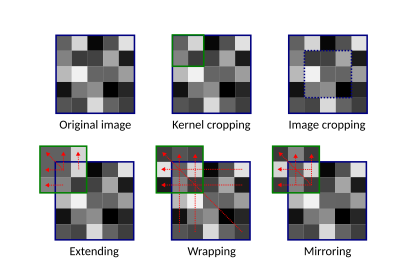
Edge pixels
You may be wondering what to do with pixels at the edge. After all, the top left pixel in the example above does not have a 3×3 neighborhood. There are various ways around this.
- You can crop the kernel, simply ignoring any pixel that is not there. So, you will just use smaller neighbourhoods for edge pixels.
- You can extend the image by repeating the border pixels values.
- Alternatively you can wrap the image around. When doing this, the left neighbours of the pixels in the first column will be the pixels in the last column, the top neighbours of the first row of pixels will be those in the last row and so on.
- A different solution is to mirror the image at the edges.
- Finally you can crop the image, and not apply the filter to the edge pixels. This will, however, result in a smaller output image.
The schematic below summarises these options for the top-left pixel of an image
Basic filters in Scikit Image
The Scikit Image filters submodule contains a lot of different functions to apply filters to images. The simple filters described above are found within the filters.rank submodule.
Let’s start by loading an image. This shows some cell nuclei, and is quite noisy.
from skimage.io import imread, imshow

nuclei = imread("nuclei_noisy.tif")

imshow(nuclei)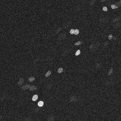
We can now apply the minimum, maximum, mean and median filters to the image
import numpy as np
from skimage.filters.rank import minimum, maximum, mean, median

img_min = minimum(nuclei, selem=np.ones((5, 5)))
img_max = maximum(nuclei, selem=np.ones((5, 5)))
img_med = median(nuclei, selem=np.ones((5, 5)))
img_mean = mean(nuclei, selem=np.ones((5, 5)))
The selem parameter defines the kernel as a matrix of 0 and 1. We use np.ones to define a $5 \times 5$ matrix of 1. We can use this to use kernels that are not square for example selem = np.array[[0,1,0], [1,1,1], [0,1,0]] (or you can use Numpy functions such as np.diamond, or, np.disk).
Here is what we get
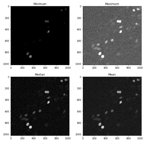
In general, the minimum filter acts as a “shrinking” filter, while the maximum filter expands object borders. This are useful, for example, when detecting objects in an image.
The mean and median filter are good at removing noise, by eliminating the effect of very bright or very dark pixels; usually the median filter works better, and is often used at the beginning of many image analysis pipelines.
Convolutional filters
Similar to what discussed above, convolutional filters can be used to process images.
Convolution takes each pixel of the image, together with its neighbours, and adds them together, weighting the sum by the value of a kernel of the same size of the neighbourhood. The kernel can be of arbitrary size, and its values should generally sum to 1. So, for instance, having the following image and kernel
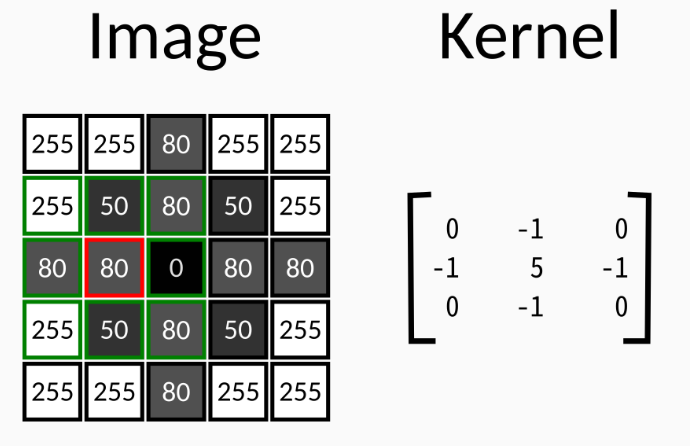
The output value for the pixel marked in red will be
$$255 * 0 + 50 * (-1) + 80 * 0 + 80 * (-1) + 80 * 5 + 0 * (-1) +$$
$$255 * 0 + 50 * (-1) + 80 * 0 = \mathbf{220}$$
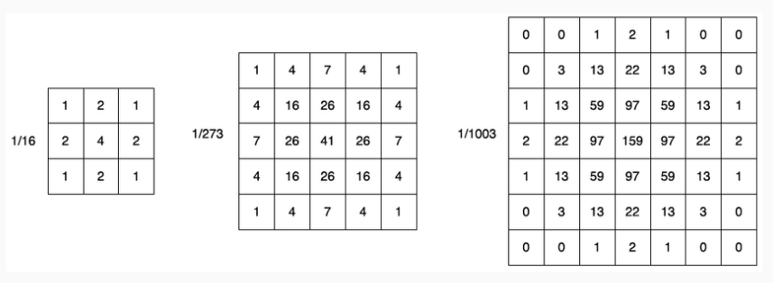
A very commonly used convolutional filter is the Gaussian filter. Some examples of Gaussian kernels are shown here
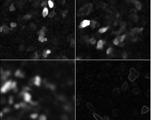
The Gaussian filter has the effect of blurring the image. For example
from skimage.filters import gaussian

# 5x5 kernel
imshow(gaussian(nuclei, sigma=5))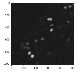
Subtracting the blurred version of an image from the original one, and adding back to the original has the effect of actually sharpening it! This filter is called unsharp mask, and is available in skimage.filters. The radius parameter is the kernel size for the Gaussian smoothing, and amount is a multiplier. The output of the filter is
$\text{output} = \text{original} + \text{amount} * (\text{original} – \text{blurred})$
from skimage.filters import unsharp_mask

nuclei_sharp = unsharp_mask(nuclei, radius=10, amount=1)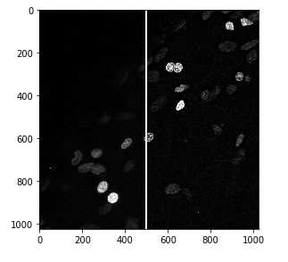
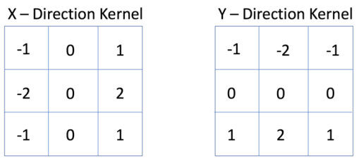
Another commonly used convolutional filter is the Sobel filter, used for edge detection. It uses two kernels, one for determining horizontal edges and one for vertical edges
from skimage.filters import sobel

nuclei_edges = sobel(nuclei)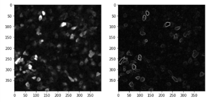
There are many other filters you can apply, I would suggest having a look at the Explained Visually where you can play with convolutional filters! I hope this post gave you a brief introduction to filters and keep an eye for new parts of this series!