Image analysis made easy with Scikit Image! (part 1)

There are lots of amazing tools for image analysis out there, to perform some really powerful and complex analyses. Sometimes, however, you may want to create automated pipelines, for example, to analyse large amounts of images, or to process a video feed in real-time.

Countless options are out there, each with its own strengths and weaknesses. In this post, I will introduce you to a great Python library called Scikit Image to load and perform basic manipulations on images.

Images as matrices

Most of the times, when you are performing image analysis, you will be dealing with raster images. These are collections of points, called pixels, with varying intensity and colour arranged in a rectangular grid, to form your image. It is therefore very convenient to represent an image as a matrix with a number of elements corresponding to that of the image pixels, and with values corresponding to their intensity.

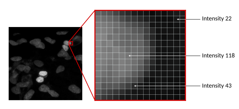
In the example below, we have an image of some nuclei, with intensity going from 0 (full black) to 255 (full white). Why 255, you ask? That depends on the bit depth of the image. This is an 8-bit image, so each pixel is represented by 8 bits; since each bit can only have 2 values (0 or 1), we have $2^8$ possible combinations. The figure below shows the range of colours for various bit depths.

Sometimes your image may have more than 2 dimensions! Maybe you are dealing with 3D microscope stacks, in which case you would store the image in a 3D matrix, or maybe you have a video or images from multiple wells of a multi-well plate. So, in general, you would use an n-dimensional matrix to store your image(s).

If you ever had to deal with matrices in Python, you have probably been using Numpy. If not, don’t worry, the next paragraph will introduce this to you, you will soon become good friends!

A very brief intro to Numpy

Numpy is a great library for numerical computing in Python. It makes it super-easy to work with n-dimensional arrays. You can easily install it through pip

pip install numpy

Let’s define a 4 by 3 array in Numpy

import numpy as np

test = np.array([[1,2,3,4],
                [5,6,7,8],
                [9,10,11,12]])

array([[ 2,  4,  6,  8],
       [10, 12, 14, 16],
       [18, 20, 22, 24]])

# Multiplication by a scalar
test * 6

array([[ 6, 12, 18, 24],
       [30, 36, 42, 48],
       [54, 60, 66, 72]])

That’s it! You can just pass a list of lists and numpy does the rest. You can then do things like

# Element-wise sum
test + test

And many more! You can refer to the Numpy website or the recently published Numpy paper for more detailed info. Today I will refer to a few Numpy functionalities, which I will introduce as we go…

But let’s go back to the topic of this post, Scikit Image!

Scikit Image, your image analysis friend for Python

Scikit Image contains a lot of different (very obviously named) submodules for image analysis. For example, the filters submodule allows you to apply filters to your images or the measure submodule to perform measures on it! We will start with the most important one, the io module, which allows you to read and write images!

If you never used Scikit Image before, you need to install it. Note that although you will import it into your program as skimage, you must install it as scikit-image, such as

pip install scikit-image

You can also refer to the Scikit Image website for more help on installing it.

# Import relevant functions
from skimage.io import imread, imshow

# Load the image
nuclei = imread('nuclei.tif')
# Show the image
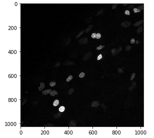
imshow(nuclei)

This shows the nuclei.tif image, saves it in the nuclei Numpy array and show it using imshow! We can inspect the resolution of the image and its bit depth by looking at the shape and dtype attributes of the Numpy array.

# Print image resolution
print(nuclei.shape)

# Print image bit depth
print(nuclei.dtype)

The shape of a Numpy array is a tuple containing the number of elements in each dimension. For example, the first print statement may return (1024, 1024), meaning that the image is a square grid of 1024 x 1024 pixels. The second print statement tells us the bit depth of the image and returns, for instance, uint8 (unsigned integer, 8-bit), meaning we have an 8-bit image.

You can show your image using different colourmaps. For example, here, I use the Viridis colourmap.

imshow(nuclei, cmap="viridis")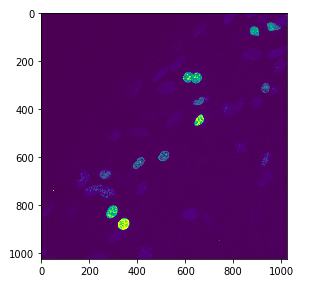

Cropping your image

One of the simplest operations you may do with your image is cropping it. This is super-easy by simply selecting the region we want in the array using Python’s indexing operator [].

# Remove 50 pixels from the left
nuclei_cropped = nuclei[:, 50:]

# Remove 100 pixels from the right
nuclei_cropped = nuclei[:, :-100]

# Remove 30 pixels around the image
nuclei_cropped = nuclei[30:-30, 30:-30]

The indexing operator also supports a step, so if you wanted to take every other row/column, you could do it like this

# Take every other row and every other column
nuclei_cropped = nuclei[::2, ::2]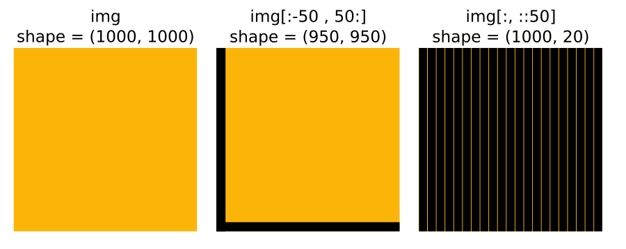

This also works with multidimensional images. For instance, if you have a 1000 frame-long movie with resolution 1024 x 1024 and you want to take only the first 100 frames you can do:

from skimage.io import imread

# Also works in multiple dimensions
movie = imread("cellsmovie.tif") # shape (1000, 1024, 1024)
movie_start = movie[1:100] # First 100 frames only

Resizing your image

Scikit Image can be used to easily resize images. There are three main functions in skimage.transform:

• rescale to scale up/down by a certain factor
• resize to scale up/down to a certain size
• downscale_local_mean to scale down with local averaging to prevent artefacts

For example, we can use rescale to increase the size of an image by 3 times

from skimage.transform import rescale

img = imread("cells.tif")

img_rescaled = rescale(img, 3, order=1)

The order parameter (valid range 0 to 5, default is 1) defines the interpolation used to generate the new pixels. A value of 0 means no interpolation (i.e. just take each pixel and generate a 3×3 grid with the same intensity). Values above 0 mean to interpolate linearly (order = 1), bi-linearly (order = 2), bi-quadratically (order =3) and so on.

We can use resize in the same way, but we specify a target shape

# Shrink the image to 100 x 100
image_small = resize(image, (100, 100))

Image histograms

One of the most common operations that you may do with images is manipulating their histogram. But let’s not get ahead of ourselves, what is an image histogram? It is simply a plot of the distribution of pixel intensities in the image.

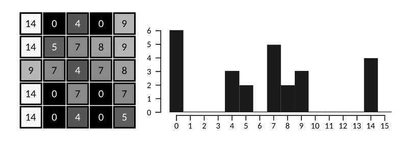
The image above shows a simple 5×5 4-bit raster image. On the right, we see the histogram, showing that there are 6 pixels with intensity 0, no pixels with intensity 1 to 3, 3 pixels with intensity 4 and so forth.
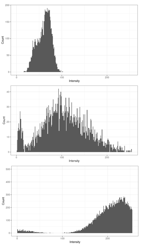
Histograms are a great way to check the quality of your image.

For instance, below are histograms for three images; the top one is underexposed, as most pixels are dark, and only a fraction of the dynamic range is used. The bottom image is overexposed; many pixels have a value of 255, which we cannot really interpret, as they may all have different brightness, but the detector on the camera was saturated and they cannot be distinguished. The middle histogram shows the best situation, where all the dynamic range of the image is used.

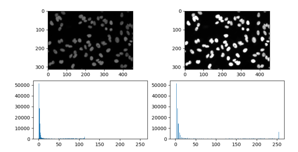
Plotting a histogram is really easy using the hist function in Matplotlib.

from skimage import imread, imshow
import matplotlib.pyplot as plt

nuclei = imread("nuclei.tif")

imshow(nuclei, cmap="gray")

plt.hist(nuclei.ravel(), bins=range(255))
plt.show()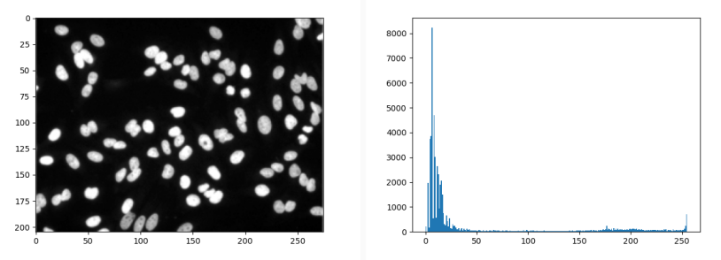

Manipulating histograms

The exposure submodule of Scikit Image has tools to manipulate image histograms, for instance in order to increase the contrast of an underexposed image.

Histogram stretching

A simple technique to increase the contrast of our image is to stretch the histogram. So, if the pixels in an 8-bit image are between 0 and 50, we are not using the possible information
between 50 and 255. If we have an image with intensity limits $m_{im}$ and $M_{im}$, and want to stretch its histogram to $m_{str}$ and $M_{str}$ we can apply the following pixel-wise

$$I_{out} = (I_{in} – m_{im})(\frac{M_{str}-m_{str}}{M_{im}-m_{im}} + m_{str})$$

This is implemented in exposure.rescale_intensity, so you don’t have to worry about coding it yourself!

from skimage.exposure import rescale_intensity

img = imread("nuclei.tif")
# Stretch the histogram!
img_stretch = rescale_intensity(img, in_range=(0, 100))

Since we may not know the input range in advance, we may use Numpy to calculate it.

import numpy as np
from skimage.exposure import rescale_intensity

img = imread("nuclei.tif")

# Get the 2nd and 98th percentile of the intensity as our range.
p2, p98 = np.percentile(img, (2, 98))

img_stretch = rescale_intensity(img, in_range=(p2, p98))

Histogram equalisation

While histogram stretching is a simple linear transformation of the histogram, equalisation increases image
contrast by spreading the most common intensity values in the image in the possible intensity range. It does so by flattening the cumulative density function (CDF) of the histogram. Given the probability of a pixel to have intensity $i$ (with $i$ between 0 and the maximum pixel value
$M$)

$$p_x(i) = p(x=i) = \frac{n_i}{n},\quad 0 \le i < M$$

The CDF is defined as

$$\text{CDF} = \sum_{j=0}^i p_x(x=j)$$

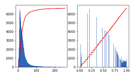
We can easily equalise the histogram of an image using skimage.exposure.equalize_hist.

from skimage.exposure import equalize_hist

img = imread("cells.tif")
img_eq = equalize_hist(img)

This is what the histogram and its CDF (the red line) look like before and after equalization.

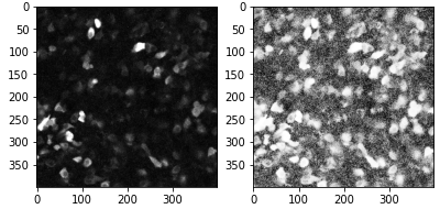
Other more sophisticated equalization strategies exist, such as adaptive histogram equalization (AHE), which computes several histograms of different image regions to improve local contrast. This tends to increase the noise in areas with low contrast. Contrast Limited Adaptive Equalization (CLAHE) solves this by reducing the amount of contrast enhancement. This is implemented in the skimage.exposure.equalize_adapthist function.

And that’s it for today! Hopefully, this post should have given you some initial insight on how Scikit Image can help with image analysis. The next part will deal with image filters, so stay tuned!