GLM for the analysis of binary outcomes

Introduction

In previous posts, I discussed how to deal with situations where you measure a continuous outcome and you want to explain its variability as a function of one or more continuous or discrete variables, using linear regression or mixed-effects models. However, there are situations where these linear models are not the best solution to use.

For example:

• The outcome variable is categorical, binary (e.g. does the subject have diabetes? Yes/No)
• The outcome is a proportion/probability (e.g. what are the odds of getting pathology A, depending on variable B?)
• Count data.

The first two cases are bounded between 0 and 1 (in the first case the variable can only be 0 or 1) or, if you prefer, 0% and 100%. In the case of count data, the outcome has a lower bound at 0 (you cannot count -20 of something!).

Linear models are very powerful, but they are problematic to use with bounded or discrete data, as they assume a continuous range of values that can assume any value from $-\infty~\text{to} +\infty$.

In this post, I will introduce generalised linear models (GLM or GLiM), a great tool you can use in those situations. As usual, we will see how to do this in R! For today we will consider the case of binary outcomes.

Some theory

Not interested in the theory? Skip directly to the code!

If you remember from my previous posts, the generic equation for a linear model is:

$$Y = \beta_0 + \beta_1 X_1 + \beta_2 X_2 + \ldots + \beta_n X_n + \epsilon$$
As said above, this equation is not good for representing bounded
data say a proportion or probability that goes from 0 to 1.
Indeed, if you were to model the proportion of patients with an illness depending on a certain parameter X with a linear model, you may end up with something like this:

$$\%\text{patients} = 0.02 + 2.5X$$

This means that if X is 50, your model will say that 125.02% of
patients are ill, which is not possible. Similarly, if X can take
negative values, you may find yourself with a negative percentage of patients. It is, therefore, necessary to introduce some non-linearity in the equation above that allows us to constrain our response, for instance, to between 0 and 1.

GLMs solve this by introducing a link function $f$ such that $f(Y)$ is a linear combination of the predictors.
$$f(Y) = \beta_0 + \beta_1 X_1 + \beta_2 X_2 + \ldots + \beta_n X_n + \epsilon$$

For instance, if $f$ is a logarithm, it will constrain the output of the model to positive numbers only, thus imposing a lower bound of 0 to our response. Note that this is still a linear model! Although the relationship between $Y$ and the predictors $X_i$ is not linear, the relationship between $f(Y)$ and $X_i$ is!

Several link functions are used, depending on the context*. Today we are going to use a binomial logit link function to model a binary outcome, which will give us a GLM called binomial logistic regression.

$$\ln(\frac{p(Y)}{1-p(Y)}) = \mathbf{X}\boldsymbol{\beta}$$

where $p(Y)$ is the probability of $Y$ happening.

Because the logit function is only defined between 0 and 1, then this is a great choice for modelling our binary variable! So, essentially, we are set to model something that looks like this

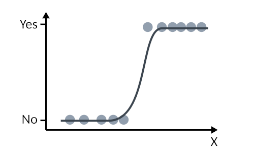
*As a note, if $f$ were the identity function $f(Y) = Y$, then we would revert to the special case of the general linear model!

Logistic regression in R!

The dataset

For this example, I am going to use the babyfood dataset from the faraway package. This is also analysed in the excellent book “Extending the Linear Model with R” by Julian Faraway. The dataset contains the proportions of children developing a respiratory disease in their first year of life in relation to the type of feeding and sex.

We will first load and visualize the data, then fit a GLM to it.

library(faraway)
babyfood

  disease nondisease  sex   food
1      77        381  Boy Bottle
2      19        128  Boy  Suppl
3      47        447  Boy Breast
4      48        336 Girl Bottle
5      16        111 Girl  Suppl
6      31        433 Girl Breast

The data has counts for each condition, let’s plot the percentage of babies with disease. We first reorder the food variable so that Breast is the reference level.

babyfood$food <- factor(babyfood$food, 
                 levels = c("Breast", "Bottle", "Suppl"))

ggplot(babyfood, aes(x = sex, 
  y = disease/(disease+nondisease)*100)) +
  geom_col(aes(fill=food), position = "dodge") +
  ylim(0, 100) +
  ylab("% disease") +
  xlab("Sex")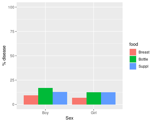

Creating a GLM

We can now fit the model using the R glm function. As explained above, we specify that we want a binomial logit link function.

model <- glm(cbind(disease, nondisease) ~ sex + food, 
             family = binomial(link = logit)
             data = babyfood)

The syntax of glm is very similar to lm. We pass a formula for the model, and we specify the link function. Note that because we do not have individual data we just pass a data frame with occurrences of disease and non-disease. If our dataset had data for individual subjects such as

 sex disease babyfood
1  M       Y   Breast
2  M       N   Bottle
3  M       N   Breast
4  M       Y    Suppl
5  F       Y   Breast
6  F       N    Suppl

we could have used

model <- glm(disease ~ sex + food, 
             family = binomial(link = logit)
             data = babyfood)

Interpreting the GLM output

Now, let’s see the output of our model

summary(model)

Call:
glm(formula = cbind(disease, nondisease) ~ sex + food, family = binomial(link = logit), 
    data = babyfood)

Deviance Residuals: 
      1        2        3        4        5        6  
 0.1096  -0.5052   0.1922  -0.1342   0.5896  -0.2284  

Coefficients:
            Estimate Std. Error z value Pr(>|z|)    
(Intercept)  -2.2820     0.1322 -17.259  < 2e-16 ***
sexGirl      -0.3126     0.1410  -2.216   0.0267 *  
foodBottle    0.6693     0.1530   4.374 1.22e-05 ***
foodSuppl     0.4968     0.2164   2.296   0.0217 *  
---
Signif. codes:  0 ‘***’ 0.001 ‘**’ 0.01 ‘*’ 0.05 ‘.’ 0.1 ‘ ’ 1

(Dispersion parameter for binomial family taken to be 1)

    Null deviance: 26.37529  on 5  degrees of freedom
Residual deviance:  0.72192  on 2  degrees of freedom
AIC: 40.24

Number of Fisher Scoring iterations: 4

The summary is similar to that of lm, with some important differences. We have an intercept that is different from 0, as this represents the basal odds of disease for the control group (breast-fed boys). We see that there are also significant effects of both gender and food type. Now, you should be very careful interpreting these coefficients because remember that we are modelling the ln(odds), so we should exponentiate them to get the odds!
So, for instance, for girls, $\hat\beta = − 0.3126$

exp(-0.3126)

[1] 0.7315425

This means that being a girl brings the odds of having a respiratory disease to 73.2%, compared to the reference level (boys). You can calculate confidence intervals for the estimates using the confint function. Remember to exponentiate them so that you can talk about odds rather than log(odds)!

exp(confint(model))

Waiting for profiling to be done...
                 2.5 %    97.5 %
(Intercept) 0.07818602 0.1313591
sexGirl     0.55362089 0.9629225
foodBottle  1.45028833 2.6441703
foodSuppl   1.06463534 2.4926583

Alternatively, you can approximate the 95% CIs
using $e^{(\hat\beta \pm 1.96 \text{SE}\hat\beta)}$. For example, for $\hat\beta_1$ we have exp (− 0.3126 ± 1.96 ∗ 0.1410) giving [0.5549041, 0.9644088], very similar to what calculated by confint. Note how these intervals are not symmetric, since we are working on a non-linear scale.

The model’s summary also reports a measure of deviance.
This is a goodness-of-fit measure useful for GLMs; in general the lower the deviance, the better. The summary reports a Null deviance of 26.38 on 5 degrees of freedom and a Residual deviance of 0.72 on 2 degrees of freedom.

The null deviance refers to the intercept-only model (essentially a null model where we say that neither sex nor feeding have an effect on the odds of disease). Since we have 6 observations, that null model has 5 degrees of freedom. Our current model adds 3 variables (1 dummy for Gender, 2 dummies for food), thus has only 2 degrees of freedom, but has a much-reduced variance, indicating that our model fits the data much better than an intercept-only model!
We can use the drop1 function to see the contribution of each model parameter.

drop1(model)

Single term deletions

Model:
cbind(disease, nondisease) ~ sex + food
       Df Deviance    AIC
<none>      0.7219 40.240
sex     1   5.6990 43.217
food    2  20.8992 56.417

Not surprisingly, we see that removing either Sex or Food from the model results in increased deviance (and an increased AIC, another goodness-of-fit measure for which, again, the lower the better.). Obviously, when looking at this type of data we always need to be very aware that many other confounding factors (e.g. socioeconomic status) may be important to consider.

Finally, a note on the “deviance residuals” that appear in the model’s summary. These are not the traditional residuals we get from lm. Deviance residuals represent the contribution of each sample to the model deviance. The sum of squares of the model residuals is the deviance!

And this is all for today, I hope you enjoyed this short intro to GLMs!