In a previous post, I discussed how to use linear regression to analyse whether one or more variables influence an outcome. Linear regression is great, but it is not always the best solution; one of the extremely important assumptions of linear regression is that the observations are independent. However, there are a lot of situations when that does not apply. This post will explore how to use mixed-effects models in R to deal with this!
Experimental designs giving non-independent measures
Not interested in the theory? Jump directly to the example!
Two of the main types of experimental design where you end up with non-independent observations are repeated measures and nested designs.
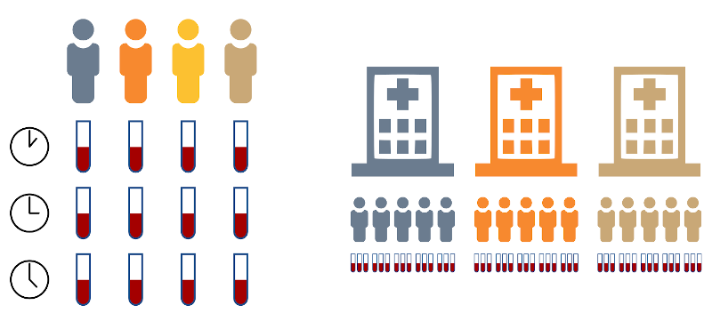
In repeated measures design, you are taking measurements from the same experimental unit multiple times; a typical example is taking multiple blood samples from the same patient over the course of several visits. Because the measures always come from the same individual, they are not independent, and they are likely to be more correlated between each other than they are with measures from a different individual.
In nested design, you are taking measurements that have some hierarchical or nested structure. For example, you may take biopsies from various patients at different clinics, and then analyse multiple cells in each biopsy. The cells coming from the same biopsy come from the same piece of tissue, thus they are not independent and may have some higher degree of correlation than cells from different biopsies. Furthermore, patients at the same clinic may also show some higher degree of correlation because they are treated by the same medical staff, using the same procedures and maybe because they live in the same area. So we have a nesting of the type clinic > patient/biopsy > cells.
Why should I bother (replication and pseudoreplication)?
So… what’s the big deal with having non-independent samples? We will see some examples below, but the issue is that we risk creating models that do not correctly represent the real variability in our sample. For instance, think about the situation on the left in the figure above. If we model those as 12 independent samples, we are assuming that there are 11 degrees of freedom in our system, which is not true, as each measurement at time 2 will be somehow related to the respective measurement at time 1.
Replication is an essential part of experimental design. We perform a measurement multiple times on multiple experimental units to increase how precisely the estimations we perform on the samples approximate the parameters of the population.
By incorrectly increasing the degrees of freedom in our model, we generate inaccurate statistical models that can misrepresent reality. The process of (maliciously or not) inflating the degrees of freedom is called pseudoreplication, and it is a well-known issue in biological and other sciences (see for example Lazic 2010 or Lazic et al. 2018). By reporting having measured 12 independent samples instead of reporting 4 independent groups of 3 non-independent samples, and analysing your data according, you are falling into the pseudoreplication trap… and bad things can happen there!
A simple example
Let’s say we measure the blood level of substance X, over the course of 3 time points in 10 people. We want to know whether time has an effect on the levels of X. I created some example data to use for this post.
Let’s have a quick look at the data
ggplot(data, aes(x=Time, y=X)) +
geom_line(aes(col=Patient))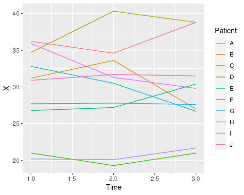
This plot tells us that time has no clear effect on the level of X, and that there is quite a bit of variability amongst patients in their X levels. This is a good example of repeated measures and one that will allow us to see the issues with pseudoreplication. So, let’s start to analyse these data using R!
The bad way
We start by creating a simple linear model to analyse our data such as:
$$X = \beta_0 + \beta_1 * Time + \epsilon$$
model <- lm(X ~ Time, data)
summary(model)
Call:
lm(formula = X ~ Time, data = data)
Residuals:
Min 1Q Median 3Q Max
-10.2700 -2.5912 0.9825 3.7788 10.7300
Coefficients:
Estimate Std. Error t value Pr(>|t|)
(Intercept) 29.980 2.879 10.413 3.91e-11 ***
Time -0.205 1.333 -0.154 0.879
---
Signif. codes: 0 ‘***’ 0.001 ‘**’ 0.01 ‘*’ 0.05 ‘.’ 0.1 ‘ ’ 1
Residual standard error: 5.96 on 28 degrees of freedom
Multiple R-squared: 0.0008443, Adjusted R-squared: -0.03484
F-statistic: 0.02366 on 1 and 28 DF, p-value: 0.8789The summary of the model tells us that Time does not influence the levels of X however, you can see that the model is representing a system with 28 degrees of freedom, which we know is wrong! Indeed, what is happening is that we are considering the measurements as all independent.
We can see this if we plot the residuals by patient
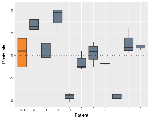
In the definition of our linear model we assume $\epsilon \sim N(0, \sigma_{\epsilon}^{2})$, which, albeit being true here when looking at all the residuals (the orange bar in the figure), it is clearly not true when looking at residuals from the single individuals. What is happening is that we are artificially inflating the sample variability, by putting the “patient effect” inside the residuals.
Let’s see if there is a better way!
The useless way
Seen that the problem lies in the individual patients we may be tempted to use it as a factor.
model2 <- lm(X ~ Time + Patient, data)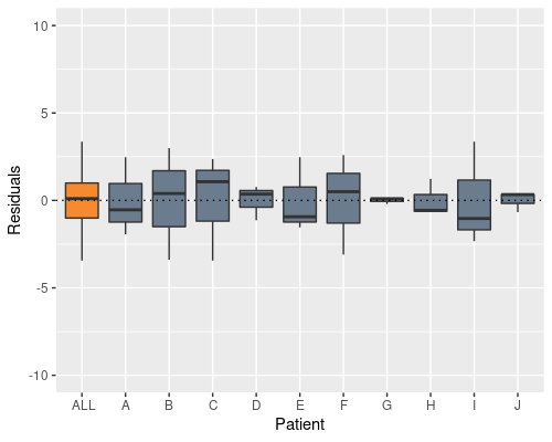
Indeed, this solves the problem, and now the patient effect is not in the residuals anymore, however the model summary raises a different issue
Call:
lm(formula = X ~ Time + Patient, data = data)

Residuals:
    Min      1Q  Median      3Q     Max
-3.4383 -1.0083  0.1025  0.9967  3.3617

Coefficients:
            Estimate Std. Error t value Pr(>|t|)
(Intercept)  36.9433     1.6598  22.258 4.52e-15 ***
Time         -0.2050     0.5082  -0.403 0.691176
PatientB     -5.9333     1.8557  -3.197 0.004743 **
PatientC      1.4000     1.8557   0.754 0.459845
PatientD    -16.1000     1.8557  -8.676 4.92e-08 ***
PatientE     -8.4000     1.8557  -4.527 0.000231 ***
PatientF     -6.5333     1.8557  -3.521 0.002286 **
PatientG     -8.8333     1.8557  -4.760 0.000136 ***
PatientH    -15.8667     1.8557  -8.550 6.16e-08 ***
PatientI     -4.2000     1.8557  -2.263 0.035521 *
PatientJ     -5.1667     1.8557  -2.784 0.011824 *
---
Signif. codes:  0 ‘***’ 0.001 ‘**’ 0.01 ‘*’ 0.05 ‘.’ 0.1 ‘ ’ 1

Residual standard error: 2.273 on 19 degrees of freedom
Multiple R-squared:  0.9014,	Adjusted R-squared:  0.8495
F-statistic: 17.37 on 10 and 19 DF,  p-value: 1.615e-07
Indeed, the residual standard error is about 1/3 of what it was before, however, what is happening here is that we are creating a lot of dummy variables to represent the patients. So our model is something like
$$X = \beta_0 + \beta_1 * Time + \beta_2 * PB + \beta_3 * PC + \ldots + \epsilon$$
Where
$$PB = \begin{cases}& 1\text{ if Patient} = B\\ & 0\text{ otherwise}\end{cases}$$
$$PC = \begin{cases}& 1\text{ if Patient} = C\\ & 0\text{ otherwise}\end{cases}$$
And so on…
So this model is not very useful, as it only models those 10 patients and cannot extrapolate to a patient 11 unless you estimate a new variable for them, which will need measuring X for that patient. Essentially, we have created a model that tells us what we already know and cannot do anything else.
The proper way, using mixed-effects models!
So, we finally get to do things the proper way, using mixed-effects models!
The idea is that we don’t use the patient as a predictor or, in mixed-effect lingo as a fixed effect, but rather like a random effect, a random variable, independent from the residuals, which influences our outcome but that we are not interested in determining. In other terms
$$X_{kij} = \beta_0 + \beta_1 * Time + b + epsilon$$
Where we have 10 random effects $b \sim N(0, \sigma_b^{2})$, each of which is shared by the 3 measurements from each patient, plus 30 residuals $\epsilon \sim N(0, \sigma_{\epsilon}^{2})$, one per observation.
Unfortunately, lm cannot handle mixed-effect models, so we need to use the lme function in the nlme package.
library(nlme)

model3 <- lme(X ~ Time, random=~1|Patient, data)
The syntax of lme is essentially the same as lm, plus a random term, which I will explain below.
summary(model3)

Linear mixed-effects model fit by REML
 Data: data
       AIC      BIC    logLik
  166.4679 171.7967 -79.23394

Random effects:
 Formula: ~1 | Patient
        (Intercept) Residual
StdDev:    5.611054 2.272793

Fixed effects: X ~ Time
             Value Std.Error DF   t-value p-value
(Intercept) 29.980  2.086551 19 14.368206  0.0000
Time        -0.205  0.508212 19 -0.403375  0.6912
 Correlation:
     (Intr)
Time -0.487

Standardized Within-Group Residuals:
        Min          Q1         Med          Q3         Max
-1.47025716 -0.48710670 -0.02399607  0.31374056  1.54213668

Number of Observations: 30
Number of Groups: 10
R has correctly identified that we have 30 observations but only 10 experimental units! The rest of the summary is pretty much the same as for lm, however instead of getting $R^2$ as a goodness-of-fit measure we get three measures, AIC, BIC and log-likelihood. Briefly, lower values of AIC or BIC, or higher value of log-likelihood indicate a better fit.
Random intercepts and random slopes
So, what exactly is happening here? Let’s look at the estimated coefficients
> coef(model3) (Intercept) Time
A 36.58225 -0.205
B 30.95659 -0.205
C 37.90966 -0.205
D 21.31711 -0.205
E 28.61783 -0.205
F 30.38770 -0.205
G 28.20697 -0.205
H 21.53834 -0.205
I 32.60004 -0.205
J 31.68350 -0.205R is estimating a different intercept for each patient, whilst keeping the same slope for Time. We have created a random-intercept mixed-effects model.
Why does it only change the intercept? That is because we defined the random effects as ~1 | Patient. This tells R we want to estimate a different intercept (indicated by 1) for each patient. We can also estimate different slopes for the different fixed effects in our model, by specifying them in the random effects formula. For instance
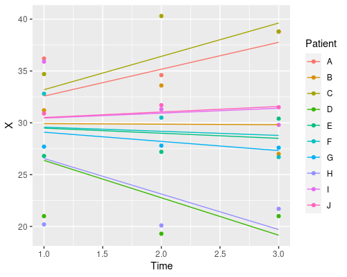
model4 <- lme(X ~ Time, random=~Time|Patient, data)
coef(model4)
(Intercept) Time
A 34.98618 0.66094525
B 32.97207 -1.20892331
C 35.51697 1.07422047
D 21.09373 -0.17600178
E 26.48515 0.85413897
F 33.41293 -1.72205606
G 28.04105 -0.13863582
H 20.51766 0.22698304
I 35.62665 -1.70147529
J 31.14762 0.08080454Similarly, if we wanted a random slope model, where we change only the slope and not the intercept we would use ~Time-1 | Patient.
Finally, let’s plot the model’s prediction in the three situations
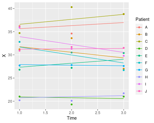
ggplot(data, aes(Time, X)) +
  geom_point(aes(col=Patient)) +
  geom_line(aes(x = Time, y = predict(model3), col=Patient))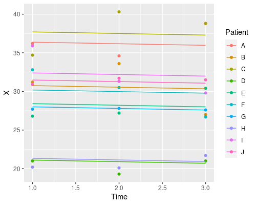
Each patient has its own intercept, the slope for time is always the same.
So, which one should I choose? Random intercept, random slope, or both? It depends on your particular problem, and this is where domain-specific knowledge comes into play. Which model makes more sense in biological terms?
Mixed-effects models are a much more complex topic and there is much more you can do with them, two good reference books are “Mixed Effects Models in S and S-PLUS” by Douglas Bates and José Pinheiro and “Extending the Linear Model with R” by Julian Faraway.
And that is all for today, hope you enjoyed this post!
6 replies on “A gentle introduction to mixed-effects models”
Thank you! Excellent blog!
Interesting to summarize assumption for data ( independence etc) and for residuals ( normality etc)
Keep posting !
Thank you Manoel! Glad you enjoyed it!
Other posts will be coming soon!
really great article, thanks!
in the 1st sentence of the 1st paragraph, you missed the “non-” before “independent”, right? might be confusing to some readers…
Well spotted Nico! I have now corrected the text, thank you.
Thanks for this. A small correction on the Pseudoreplication in the top ‘grey backgound’ text.
Thanks once more.
Thank you Jacob!