In today’s post, we are going to perform some sample classification using machine learning in R. We are going to use a publicly available dataset, the Breast Cancer Wisconsin (Diagnostic) Data Set (WDBC), which is available on the UC Irvine Machine Learning Repository. This is a fairly simple dataset, which is good to get started on this topic. We are going to use one of the simplest machine learning algorithms, binary trees.
Data import
The WDBC dataset contains data extracted from micrographs of fine-needle aspirates of breast masses. The images have been analysed to define a series of features describing the nuclei of the cells in the image. The data descriptor gives more extended information (always read data descriptors when available!).
The first thing we need to do is to import the data. R is able to read the data directly from the UCI URL. Note that the file is missing the column names, so we need to specify header = FALSE
wdbc <- read.csv("https://archive.ics.uci.edu/ml/machine-learning-databases/breast-cancer-wisconsin/wdbc.data",
header = FALSE)
We can refer to the data descriptor to see what each column is, and add the names to our data. There are 10 features reported as mean, standard deviation and maximum for each image.
# The names of the features, as per the data descriptor
features <- c("radius", "texture", "perimeter", "area",
              "smoothness", "compactness", "concavity",
              "concave_points", "symmetry",
              "fractal_dimension")
# Assign the names of the features to the column names
# plus id and diagnosis for column 1 and 2
colnames(wdbc) <-
c("id", "diagnosis",
  paste0("mean_", features),
  paste0("sd_", features),
  paste0("max_", features))
Exploratory analysis
There are a lot of predictors in this dataset, we can try plotting a few to get a better idea of our dataset.
I am going to pick a few random features and plot them for the two groups that we are trying to distinguish
library(ggplot2)

ggplot(wdbc, aes(mean_symmetry)) +
  geom_density(aes(fill=diagnosis), alpha=0.3)

ggplot(wdbc, aes(mean_radius)) +
  geom_density(aes(fill=diagnosis), alpha=0.3)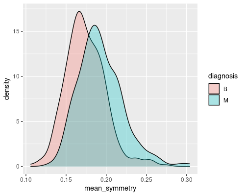
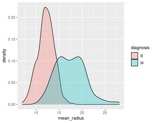
These are two good examples of a feature that gives a decent discriminatory power (mean radius) and of one that is less interesting (mean symmetry). Indeed, you can imagine that if you just had the radius you would be able to tell most of the times whether a tumour is malignant or not. For example, if the radius is greater than 15 there is a high chance that the tumour is malignant.
Plotting more than one feature at a time may prove even more useful
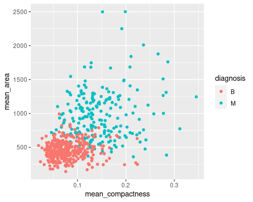
In this case, we can see an almost straight border between the two classes, making it easier for us to distinguish the two groups. You can imagine that visualising this in a higher dimension space (for example the 30-features space of our dataset) may prove even more useful.
Data preparation
Binary trees are a method of supervised learning. In these methods, we train a classifier using some labelled data, and can then use it to predict the outcome on some new, unlabelled data. Before creating our binary tree, however, we will divide our data into a training and a test set. We will use the training set for creating the classifier and we will test its accuracy on the test set. In this way, we will avoid what is called overfitting; this means that we avoid creating a classifier that is really good at predicting the training data but is not able to extrapolate the results to a new set of observations.
A note on normalisation: binary trees are not influenced by normalisation of the variables; many other classification methods (especially those that take into account distance between samples) do require normalisation so that variables that contain bigger values are not over-influencing the classifier. If using those classifiers you should therefore normalise your variables first, for example by scaling them between 0 and 1 or by scaling them so that their mean is 0 and their standard deviation is 1.
Training and test set
Splitting our dataset is extremely easy. We use the sample function, to randomly sample data points. sample is one of many R functions that uses randomly generated data. To ensure reproducibility of these examples we will use the set.seed function that initialises the pseudo-random number generator in R using a certain seed value.
# You can use any number you like as a seed If you use
# 46 you will get the same results as me, otherwise
# results are very likely to be different
set.seed(46)
num.samples <- nrow(wdbc)

# We sample 80% of the values from 1 to num.samples and
# choose the corresponding lines as the test set
test.id <- sample(1:num.samples, size = 0.8 * num.samples,
                  replace = FALSE)
# The training set consists of all the samples that are
# not in the test set
wdbc.test <- wdbc[test.id,]
wdbc.train <- wdbc[-test.id,]
We can check the number of samples in the training and test sets.
nrow(wdbc.train)[1] 114nrow(wdbc.test)[1] 455Binary trees
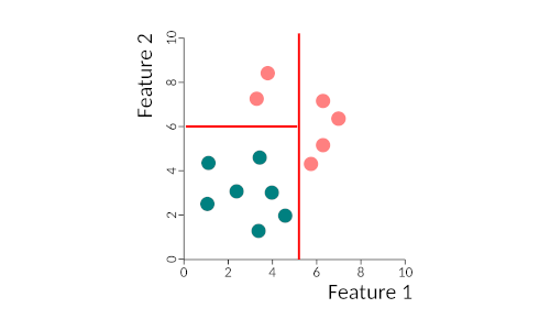
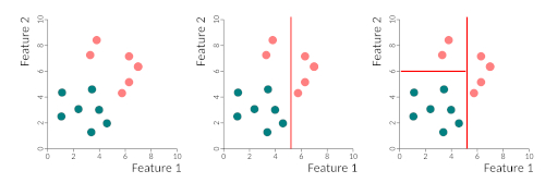
Binary trees work by partitioning data into two subsets, in a recursive way, until all data is classified. What happens is that we find the best discriminatory feature and separate the two classes using that feature. Then it takes the two sub-spaces and partitions each one according to the best-predicting features, and so on either until all samples are correctly classified or until some stop criteria that we can specify. This figure gives you a very simple example of the partitioning of space by a binary tree. We first separate the two classes by feature 1, then we re-partition the left side by feature 2. The right-hand side does not need repartitioning. The tree could be written as:
- if feature 1 > 5 then class = pink
- else if feature 1 < 5 and feature 2 > 6 then class = pink
- else class = blue
Creating the tree
Let’s see this in action on our dataset. We use the rpart library to create the tree and the rpart.plot library to visualise it.
library(rpart)
library(rpart.plot)

# Predict diagnosis using all of the other classifiers,
# indicated by . but do not use the id, as that is not an
# useful classifier.
tree <- rpart(diagnosis ~ . -id, data = wdbc.train)
We can visualise the tree in a textual manner or use the rpart.plot function to plot it.
print(tree)n= 114
node), split, n, loss, yval, (yprob)
* denotes terminal node
1) root 114 50 B (0.56140351 0.43859649)
2) max_perimeter< 101.7 56 0 B (1.00000000 0.00000000) *
3) max_perimeter>=101.7 58 8 M (0.13793103 0.86206897)
6) max_texture< 23.74 5 0 B (1.00000000 0.00000000) *
7) max_texture>=23.74 53 3 M (0.05660377 0.94339623) *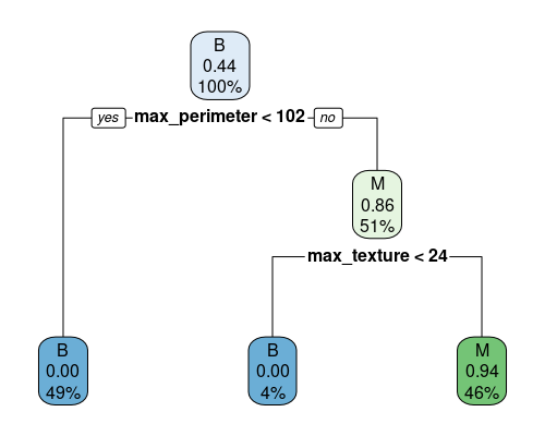
This is very straightforward to read. We start at the top and go down. The top node contains all samples (100%), and the plot tells us that the majority are of class B, and that at this point the predicted probability for the M class is 0.44, since we have 50 M over 114 total samples. We then split by max_perimeter. If it is less than 102 (49% of samples), we definitely classify samples as B, with a probability of classifying the sample as M of 0. On the right, we need two other splits to finish our classification.
This vignette gives extensive notes on how to personalise the tree plot.
Model evaluation
So, how good is our model? We can ask it to predict what the test set should be and check whether it gives us the correct answers!
test.pred <- predict(tree, newdata = wdbc.test,
                     type = "class")
conf.mat <- table(wdbc.test$diagnosis, test.pred)
print(conf.mat)
test.pred
B M
B 277 16
M 33 129The table above is called a confusion matrix and it gives us an idea of the accuracy of our tree. We can see that out of 293 benign tumours in the test set, 277 are classified correctly. For malignant tumours, where 33 out of 162 are wrongly classified. We can calculate the model accuracy by dividing the sum of the numbers in the diagonal (correctly classified) by the total of samples.
acc <- sum(diag(conf.mat))/sum(conf.mat)
print(acc)
[1] 0.8923077Note that if we were to calculate accuracy on the test set, it would generally be higher (in this case ~97%); however this is not really a useful measure, as the tree has been generated using that data, and so it is biased towards it (overfitting). An accuracy of 89% is not too bad, however, we can probably do better!
Cross-validation
One important step to decrease the chances of overfitting is to use cross-validation (CV). We perform the training on many different subsets of the data set. So, if we had 200 observations, we may use 150 (3/4) to train the dataset. By changing which 1/4 of the data to use as a test set we would be performing 4-fold CV.
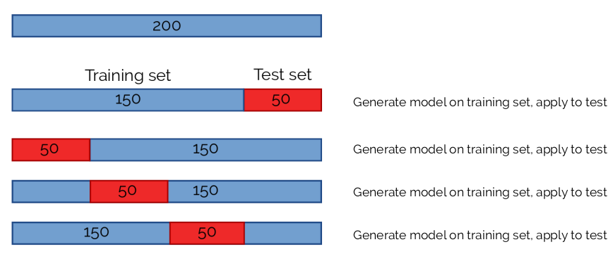
It is common to perform 5- or 10-fold CV, and in some cases, people use “leave-one-out” CV, where only 1 element is used at a time as a test set.
We will perform 10-fold CV using the caret package.
library(caret)

# Define the parameters for 10-fold CV
train.control <- trainControl(method = "cv", number = 10)
# Create the trees
tree.cv <- train(diagnosis ~ . -id, data = wdbc,
                 trControl = train.control, method='rpart',
                 tuneLength = 10)
The train function in caret will automatically perform CV for us. Note that this function can be applied to many other models, not just binary trees, by changing the method parameter. The tuneLength parameter will try different values of the main parameters for the method that we use, further optimising the output. In the case of rpart it will change the cp parameter of the tree, which controls how complex our binary tree is (e.g. number of splits and nodes). We have asked caret to test 10 values of cp.
print(tree.cv)CART
569 samples
31 predictor
2 classes: 'B', 'M'
No pre-processing
Resampling: Cross-Validated (10 fold)
Summary of sample sizes: 512, 512, 512, 512, 511, 512, ...
Resampling results across tuning parameters:
cp Accuracy Kappa
0.00000000 0.9225845 0.8321902
0.08805031 0.8979907 0.7719623
0.17610063 0.8979907 0.7719623
0.26415094 0.8979907 0.7719623
0.35220126 0.8979907 0.7719623
0.44025157 0.8979907 0.7719623
0.52830189 0.8979907 0.7719623
0.61635220 0.8979907 0.7719623
0.70440252 0.8979907 0.7719623
0.79245283 0.7757281 0.4316902
Accuracy was used to select the optimal model using the largest value.
The final value used for the model was cp = 0.We can see that larger complexities eventually decrease accuracy (you can plot the model to see this in a graph) and a value of 0 for cp is optimal. Let’s have a look at the confusion matrix!
conf.mat.cv <- table(wdbc$diagnosis, predict(tree.cv, wdbc))
acc.cv <- sum(diag(conf.mat.cv))/sum(conf.mat.cv)
print(conf.mat.cv)
B M
B 352 5
M 17 195print(acc.cv)[1] 0.9613357Cross-validation has increased our accuracy to 96%, a much better result!
That is all for today, I hope you enjoyed this simple introduction to binary trees!