The second part of this series of posts will tackle multiple regression, that is, linear regression with more than one predictor. If you are not familiar with simple linear regression and have not read part 1 be sure to check that out first!
Introducing multiple predictors
In this post, we will extend the dataset from part 1. This CSV file contains core body temperature data for 80 subjects and gives us information about their age, weight and sex. This time we want to ask whether age, weight and sex have an effect on core body temperature. The idea is very similar to what we saw in part 1, but this time we will use linear regression to take into account more than one variable.
Exploring the data
Before we dive into linear regression and how to do it in R, let’s start with a little exploration of the data. Although this part may seem trivial, it is extremely important, to evaluate the quality of our data, check for any missing data points, outliers etc.
At this point is also important to use your own domain-specific knowledge; for example, you may know that core body temperature is extremely well regulated in the body, so you should expect a fairly small range of temperature (which is the case here).
temp <- read.csv("temp2.csv")
summary(temp)
      Age        Sex        Weight       Temperature
 Min.   :18.00   F:46   Min.   :46.00   Min.   :36.53
 1st Qu.:28.25   M:34   1st Qu.:62.00   1st Qu.:36.56
 Median :50.50          Median :68.50   Median :36.60
 Mean   :48.39          Mean   :68.58   Mean   :36.59
 3rd Qu.:65.50          3rd Qu.:75.25   3rd Qu.:36.62
 Max.   :79.00          Max.   :92.00   Max.   :36.66
This already, tells us that this is a fairly balanced dataset, as far as Sex is concerned, as men and women are (almost) equally represented. We have a fairly large range of Age and Weight, which is not a bad thing since we want to look at the effect of these variables. Let’s do some plotting!
ggplot(temp, aes(Age, Temperature)) +
geom_point(aes(col=Sex))
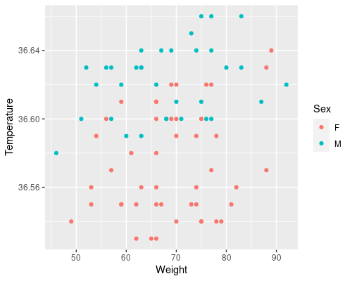
ggplot(temp, aes(Weight, Temperature)) +
geom_point(aes(col=Sex))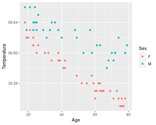
These plots tell us a lot.
- There seems to be a clear effect of age on temperature, as we saw before
- This effect looks more prominent in women than in men
- Looks like a weight has a smaller effect on temperature
- Overall, women have a lower core body temperature compared to men
Creating the model in R
OK, so how do we test all of this using linear regression? Let’s start by adding Weight to our model. Essentially we are trying to model
$$Temperature = \beta_0 + \beta_1 * Age + \beta_2 Weight$$
This is an easy extension of the equation we saw in part 1 for simple regression. Now, let’s do the same thing for sex. This is tricky! How do we plug ‘M’ or ‘F’ in an equation? The trick is to use a dummy variable. We can define $S$ as
\begin{cases}& S=0\text{ if } Sex= F\\ & S=1\text{ if } Sex= M\end{cases}
Our model thus becomes
$$Temperature = \beta_0 + \beta_1 * Age + \beta_2 Weight + \beta_3 S$$
In this example, Sex is a factor with two levels (M and F). Sometimes you may have multiple levels; for instance, considering how severe is an illness you may have a factor with levels mild, medium, and severe. In this case you would use 2 dummies
\begin{cases}& D_1=0\text{ if } Sev=Mild\\ & D_1=1\text{ otherwise }\end{cases}
\begin{cases}& D_2=0\text{ if } Sev=Medium\\ & D_2=1\text{ otherwise }\end{cases}
Luckily for us, R does all of this under the hood, so there is no need to learn new commands or to do anything fancy, we just use lm!
model <- lm(Temperature ~ Age + Sex + Weight, data = temp)By using Age + Sex + Weight in our formula, we are telling R to consider all three variables when building the model. If we inspect the model, we can see that R has indeed created a dummy variable for sex (note that we should always check that assumptions are met before looking into the model’s results; I leave that as an exercise to the reader 🙂 ).
Interpreting the model
summary(model)Call:
lm(formula = Temperature ~ Age + Sex + Weight, data = temp)
Residuals:
Min 1Q Median 3Q Max
-0.0124158 -0.0044763 -0.0002464 0.0044818 0.0120549
Coefficients:
Estimate Std. Error t value Pr(>|t|)
(Intercept) 3.657e+01 5.401e-03 6771.90 <2e-16 ***
Age -1.254e-03 3.700e-05 -33.89 <2e-16 ***
SexM 4.516e-02 1.511e-03 29.90 <2e-16 ***
Weight 9.211e-04 7.465e-05 12.34 <2e-16 ***
---
Signif. codes: 0 ‘***’ 0.001 ‘**’ 0.01 ‘*’ 0.05 ‘.’ 0.1 ‘ ’ 1
Residual standard error: 0.006657 on 76 degrees of freedom
Multiple R-squared: 0.9674, Adjusted R-squared: 0.9661
F-statistic: 751.9 on 3 and 76 DF, p-value: < 2.2e-16Interpreting a linear regression model with multiple predictors is essentially the same as what we saw in part 1, but we should spend a word on the interpretation of the estimates.
The intercept (36.57) corresponds to the temperature when all continuous variables are 0 and at the reference level for discrete factors. In our case, Sex is a factor with two levels (M and F) and the reference level is F. Why F? Because R orders levels alphabetically! If we wanted to check the order of levels we could do
levels(temp$Sex)[1] "F" "M"We could also use the relevel function, should we want to change the order.
The coefficients for Age (-0.0013) and Weight (0.00092) are interpreted as we saw in part 1: there is a decrease in 0.0013 degrees per years of age and an increase of 0.00092 per kg of weight. The coefficient for Sex (0.0451) is slightly different; because Sex is a discrete variable, this indicates an offset, for the case Sex = M (R writes the variable as SexM). So, for males, temperature will be 0.0451 higher.
Using the model to predict!

So far, we have seen how linear regression can help in determining whether a predictor influences an outcome. However, we can also use linear regression for prediction.
For example, if we had a 63-year-old woman, who weighs 65 kg our model will predict her weight to be:

Obviously, we don’t need to calculate this manually every time; we can use the R predict function to do this for us.
predict(model, newdata = list(Age=63, Sex="F", Weight=65))36.55032 Note that the prediction is slightly higher than our manual result, but that is just because of rounding error.
This is all nice and fun, but there is a problem. Remember when we plotted the data at the beginning? We noted that the effect of temperature looks more prominent in women than in men. This means that, when considering data from women we should expect a larger slope for Age, compared to data from men. However, here we only have one slope for age (-1.254e-03)! So our model is not able to capture the subtleties of our real data.
Yes, I hear you saying, we have an estimate for SexM as well… But that is not a slope, just an offset!
Enter interactions
The issue we just noticed can be solved by introducing an interaction term in our linear model. This is as simple as writing
model2 <- lm(Temperature ~ Age + Sex + Age:Sex + Weight,
             data = temp)
The Age:Sex term denotes an interaction; it tells our model to change the slope for age depending on Sex. You can add as many interaction terms as you want, even between multiple variables (e.g. Age:Sex: Weight); however multiple complex interaction terms may be difficult to interpret, so be cautious.
R also allows a shortcut to write interactions; by using the * sign between two variables you avoid having to spell out the interaction directly. The following code is equivalent to the one above
model2 <- lm(Temperature ~ Age * Sex + Weight, data = temp)Interpreting interactions
Let’s now explore the result of our model
summary(model2)Call:
lm(formula = Temperature ~ Age * Sex + Weight, data = temp)
Residuals:
Min 1Q Median 3Q Max
-0.0072738 -0.0028123 0.0001552 0.0023645 0.0063965
Coefficients:
Estimate Std. Error t value Pr(>|t|)
(Intercept) 3.659e+01 3.102e-03 11796.019 < 2e-16 ***
Age -1.501e-03 2.620e-05 -57.290 < 2e-16 ***
SexM 1.844e-02 2.055e-03 8.972 1.69e-13 ***
Weight 8.458e-04 3.968e-05 21.317 < 2e-16 ***
Age:SexM 5.554e-04 3.938e-05 14.106 < 2e-16 ***
---
Signif. codes: 0 ‘***’ 0.001 ‘**’ 0.01 ‘*’ 0.05 ‘.’ 0.1 ‘ ’ 1
Residual standard error: 0.003506 on 75 degrees of freedom
Multiple R-squared: 0.9911, Adjusted R-squared: 0.9906
F-statistic: 2083 on 4 and 75 DF, p-value: < 2.2e-16Yay! Our interaction term is there! You should be now familiar with how to read these summaries, but there are some important things you should note.
- The coefficients are different from the previous model. This is normal, correct, and expected!
- The interaction term acts as a conditional offset on the slope. We add $5.54 \cdot 10^{-4}$ degrees to the slope if
Sex=M. - If you look at the p-value for the interaction term, you can determine whether you have a statistically significant interaction. In this case, you do. If this is the case, you should not look at the p-values for the main terms (Age and Sex) anymore, as they become very difficult to interpret in this situation.
- If the coefficient for the interaction is not different from 0 (you can judge that from the p-value) then you can drop the interaction term and revert to a simpler model.
To better understand this output, let’s predict the temperature for a 42 year old man, who weights 82 kg.

And, indeed (again with a minor rounding error)
predict(model2, newdata = list(Age=42, Sex="M", Weight=82))36.63798Interactions or no interaction?
So, how do I know whether to include an interaction?
- Plot your data!
- Use an interaction plot
- Ask yourself whether it is meaningful to have one
We have already plotted the data, and suspected an interaction was present.
An interaction plot can help us graphically defining whether there is an interaction. R has a useful interaction.plot function you can use, although I do prefer using the emmip function in the emmeans package, which gives a prettier output! The emmeans package calculates the estimated marginal means (EMM) for the model that is, the mean response for each factor, adjusted for the other variables in the model. The emmip function plots an interaction plot based on these EMM (the base R interaction.plot function uses the raw data points, and does not use a linear model instead).
Let’s see an example
library(emmeans)
# cov.reduce = range is necessary because Age
# is a continuous variable. If we do not put this
# we will just see the response at the mean value for Age
emmip(model2, Sex ~ Age, cov.reduce=range)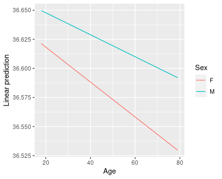
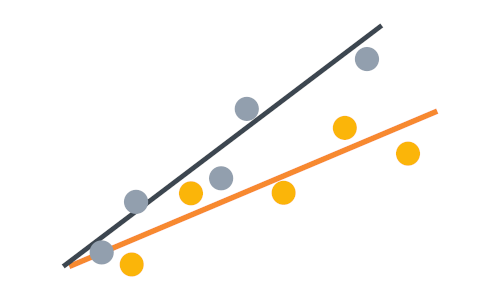
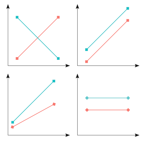
This tells us that, depending on the level of the Sex variable, the slope for Age is different. This indicates the presence of an interaction. In general, if the two lines are not parallel, there may be an interaction, like in the two panels on the left below.
In summary, interactions are a very powerful tool to add to your linear models, but be careful not to overdo it… you risk unnecessarily complicating your model a lot, and making it uninterpretable!
That is all for today, I hope you enjoyed this post and keep an eye open for new ones!